Prediction of the State of the Cardiovascular System based on the Allocation of the Boundaries of the Implementation of the Dynamic System

Minimal cCoverage and Fractality Index

This dimension is introduced by Hausdorff by the formula

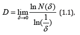
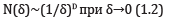
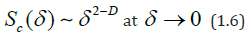
where N (δ) is the minimum number of balls of radius δ covering the set A. The basis for the definition (1.1) is the asymptotics for δ, which is defined by the expression for fractal sets.

The fractal dimension of the time series can be calculated directly through the cell dimension D_c, which is also called the Minkowski dimension or the box dimension [20].

To determine the value of D, the plane on which the time series graph is defined is divided into cells of size δ, and the number of cells N (δ) is determined, where at least one point of this graph is located. It is then constructed by the points 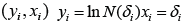regression y = ax + b , whose coefficients are estimated using the least squares method (MHK). Then is the MHK-estimate of the coefficient a. However, to reliably calculate D_c in this way, a too large representative scale containing several thousand data is required [21]. Within this scale, a time series can change many times the nature of its behaviour.

In order to associate the dynamics of the process corresponding to the series { X(t_i )} , with the fractal dimension of this time series, it is necessary to determine the dimension D locally. For this, it is necessary to find an approximation sequence that is optimal in a certain sense for each fixed δ. For this purpose, the following procedure for minimal coverages is proposed in [3]. To calculate from the fractal dimension of a time series, or the graph of a real function of one scalar variable y = f (t) , defined on a certain interval [a, b], you can directly use the procedure for determining cell dimensions, considering cell coverage as a special case of covering with rectangles.

We introduce a uniform partition of the segment [a, b] by the points

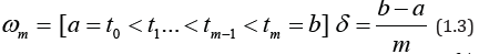
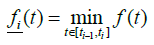
and construct the graph coverage of the function y = f (t) with rectangles with base δ and height A_i(δ) , (Figure 1) [19].

Figure 1: Fragment of cellular (gray rectangle) and minimal (black rectangle) coverings of the graph of the fractal function on the segment [t_(i-1),t_i ]. Obviously, the minimum coverage is more accurate cellular

Here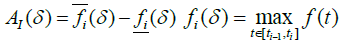

We introduce further the value

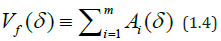
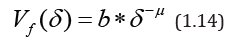
and we call V_f(δ) the amplitude variation of the function f(t) corresponding to the partition scale δ. The total coverage area Sμ(δ) is written as

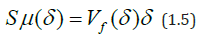
It is obvious that Sμ (δ ) is the minimum area of the graphics coverage of the class of coatings with rectangles. Therefore, such a coating is called minimal [19].

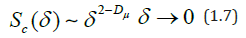
After multiplying both parts in (1.2) by δ² , for the cell division area S_C(δ) we get

and in particular for rectangular coverings

From (1.5) and (1.7) we find

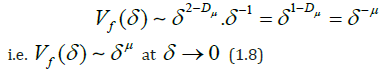
where

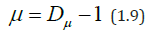
The index μ is called [19] the fractality index, and the dimension Dμ is the dimension of the minimum coverage. The value of μ is related to the stability of the time series: the more stable the behavior of the original series (i.e., oscillations occur near one level), the greater the value of μ, while the opposite is true.

If the function f(t) is called stable (quasistationary) on the interval (a, b), when its volatility is invariant on this interval, which has long been evaluated [22] by the standard deviation of changes in the selected time window (a, b), then the degradation point time series, i.e. The point at which stability is violated (quasistationarity) can be determined by the jump in volatility. For the evaluation, change in volatility points that divide the original time series into quasistationary portions (segments) corresponding jumps volatility functions developed [18] computing segmentation procedure generalizes iterative method centered cumulative sum of squares (ICSS) [23]. In general, the problem of segmentation, non-stationary time series, i.e. splitting it into non-intersecting adjacent fragments that will be statistically homogeneous (or at least possess this property in a general degree than the initial data) is known as the task of finding the chance-point problem [24,25].

The main advantage of the fractality index μ compared to other fractal indicators (in particular, with the Hurst index H) is that the corresponding value V_f(δ) has a quick access to the power asymptotic mode (1.7). The Hurst index H is determined based on the assumption that

Angle brackets here mean averaging over the interval (a, b). For comparison of μ and H, we introduce the definition of the average amplitude on the partition (1.3)

Multiply (1.4) by and substitute it into (1.8). Then we get

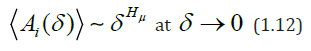
As is known [26], if f(t) is a realization of a Gaussian random process, then the Hurst index H is related to the dimension Dμ and therefore to the index μ by the relation

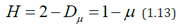
Therefore, in this case H = H_μ =1-μ . However, real physiological time series, generally speaking, are not Gaussian and therefore Hμ and H can vary greatly. Indeed, in formula (1.12) a power law holds for the average amplitude of the function f(t) over an interval of length δ, while in equation (1.10) the power law holds for the average difference between the initial and final value f(t) on the same interval. So, in general, H ≠ H_μ .

The aforementioned property of the rapid output of ( ) f V δ to the power asymptotic mode makes it possible to use μ as a local characteristic that determines the dynamics of the original process, because the representative scale for its reliable determination can be considered to have the same order with the characteristic scale of the main process states. It is natural to introduce the function μ(t) with the values of μ defined on the minimum interval μ τ preceding t. At this interval, the value of μ can still be calculated with acceptable accuracy. Since in practice a time series always has a finite length, the interval μ τ has a finite length. When calculating the rhythmogram of the heartbeat, we have taken 24 μ τ = hours, δ = ti − ti1 =1hour, b-a = 30x24 = 720 hours, m = 30.

We divide the interval (a, b) of the values of the time series f(t) into intersecting intervals of length μ τ , shifted relative to each other by 1 point (i.e., by the value of δ). In each interval of length μ τ , we construct minimal coverings Пi from rectangles with bases with amplitude variation and by points construct the regression Denote by points and construct a regression. Then MHK-estimates ^ a1 and 0 a of the coefficients a and b will be obtained by

where

Denote 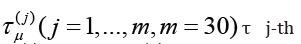j-th rolling interval length 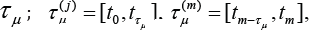and each starting point of the interval τ_μ^{( j)} let’s compare a pair of numbers b_j, μ_j .Thus, at all points we obtain the corresponding values b(t) and μ(t), defining relation (1.14). Using the resulting arrays of these values, we calculate the following characteristics: average values of μ and b values, maximum and minimum values of variation of values (variability) μ (t) and b (t). Using the resulting arrays of these values, we calculate the following characteristics: average values of μ and b values, maximum and minimum values as well as quantities and characterizing the spread of values (variability) μ(t) and b(t). Repeating the above calculations several times, we calculate the averages over all the obtained realizations of the values which will give an idea of the behavior of the local characteristics μ and b for the time series under study. Experimental studies conducted in [19] for various types of fractal time series show a low variability of the values of μ and b with a lower variability of the value of b.

Since the value of b is closely related to the distribution of the increments of the time series and, therefore, to the volatility of the time series, for to apply the computational segmentation procedure [18] based on the detection of the jump of the volatility function, it is advisable to use to divide the non-stationary series into “quasistationary” parts with the initial series f(t), the series of values of b(t) and as an estimate of the points of change of the studied series to take the average value of the points of change obtained for the original series f(t) and the number of the values of b(t), respectively.

Algorithm for Detecting Changes in Volatility

We give a brief description of the theoretical part of the method for estimating the point of change in the volatility of the time series used in [18].

Consider a time series model.

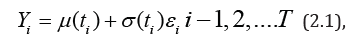
where { }i y is the sequence of random variables { }i ε is the sequence of stationary errors of observation of the quantity Y at the instants of time are the regression function (conditional average) and the volatility function (conditional variation), respectively. Model (2.1) is a special case of the non-parametric model

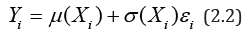
when X =t and, therefore, Хi=ti.

Following the procedure for finding a single point change (single change-point) volatility [23], we set

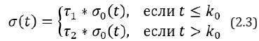
where 1 2 0 τ ,τ andk are unknown parameters. For simplicity, we put 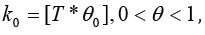, where [a] means the largest integer not exceeding a.

Let the hypothesis H0 mean that volatility has no points of change. When this hypothesis is fulfilled, it follows from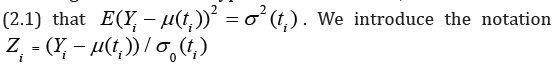

and determine the statistics

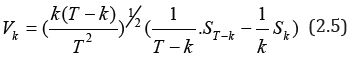
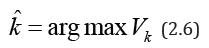
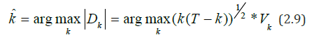
If μ (t) and 0G (t) are known, the least-squares method (MHK) for the volatility jump point k0 can be used to obtain the following estimate [27]

The value of k V will be close to 0 when the hypothesis H0 is fulfilled and is non-zero if the volatility changes. Simple calculations lead to equality

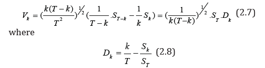
The statistics Dk, defined by the formula (2.8), differs only in sign from the statistics 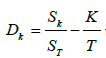used in [23]. From (2.7) it follows that Dk can also be used as an estimate of the point of change k0.

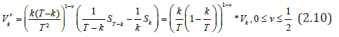
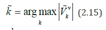
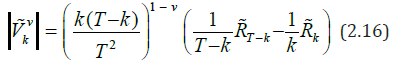
In [27], more general statistics for detecting changes in volatility are introduced.

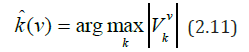
From (2.10) we can obtain an estimate for the point of change k0

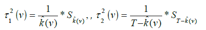
By specifying kˆ(v) one can obtain the following estimates of the quantities τ₁² τ₂²

To establish the asymptotic distribution of the statistics v k V with the known functions of regression μ(t) and conditional variation σ(t), the notation is introduced

If 1 2 τ =τ = 1 , i.e. hypothesis H0 is true, then under a certain condition [27] the limiting relation

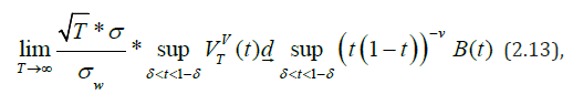
where d means convergence in distribution - any number from (0,1) 0 ≤ v ≤ 1 B(t)- standard Brownian motion by [0,1]; 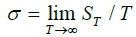and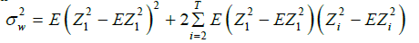

The approximation of the random variable from the right-hand side of (2.13) with ν=1/2 is obtained using the formula [28]:

If there is a jump in the volatility of the function, i.e. heteroscedastic regression model σ 2 (t) ≠ const , the estimate of the point of change is defined as [27]:

Where

μˆ (t) - evaluation of the regression function μ(t). The limiting relation (2.13) under certain conditions from [27] remains valid when kˆ (v) and k V are replaced by kˆ(v) and ˆ v k V .

To estimate 0σ (t) (2.3), it is advisable (especially when there is a certain amount of outliers or when the observation distribution function has “heavy tails”) to use the absolute deviation estimate [29]

where

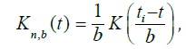
K(.)-nuclear function, and n b = b -sequence of strip widths. As a nuclear function K(t), one can adopt the standardized Epechnikov core

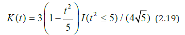
or Gauss core

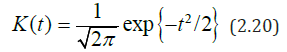
Here I(A) is an indicator function of set A:

I (A) = 1atx ∈ A and I(A)=0 at x ∉ A.

To estimate the widths of the bands in (2.18), we use the method using the , which is defined as [30]

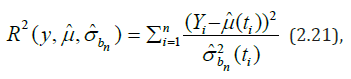
where defined by formula (2.17) with the strip width b=bn. The expected value of χ 2 - Pearson statistic (2.21), ER2, is approximately equal to the number of degrees of freedom n.

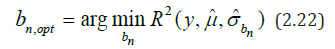
Since R2 depends on the estimated (conditional) variation, equality (2.21) can be used for the optimal choice of the bandwidth bn:

To detect the volatility points of the time series Y(t), we preliminarily construct the estimate μˆ (t) , the trend component μ(t) and allocate the irregular stochastic component a(t) = Y (t) − μˆ (t) with the property of stationarity (in broad sense) i.e. with constant mean m and covariance function 1 2 K(t , t ) , depending only on the difference of the arguments. The verification of the a(t) process for stationarity is carried out using a sample autocorrelation correlogram function [31], which for a stationary time series must rapidly decrease with increasing delay time.

Consider a stationary time series{ } t a with zero value and variances (variances) 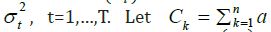be the cumulative (accumulated) sum of the series { } t a and 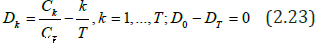centered and normalized cumulative sum of squares.

For a constant variance t σ =σ , the sequence { } k D oscillates with respect to zero. If sudden changes in the variance t σ are possible, then the graph of the dependence of Dk on k will be concluded with a high probability within certain limits, which are calculated from an analysis of the asymptotic distribution of Dk relative to some constant dispersion. Given this property, in [23] is

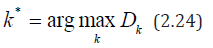
If the maximum in (2.24) exceeds the above-mentioned boundary levels k D level of significance α, then according to the iterative method of centered cumulative sums of squares (ICSS), the k* value from (2.24) is taken as the estimate of the point of variation of the variance.

In [27], a modified ICSS algorithm was proposed (let’s call it MICSS), in which the statistics D_k is replaced by v k V defined by expression (2.10). The critical values of v ( ) a v C T of the statistics k V for ν=0 are given in [23], and for ν=1/2 in [28]. For the level of significance, α=0.05 is usually applied.

In the MICSS method in step 1, the statistics

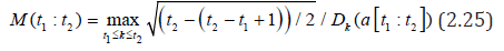
replaced by statistics

where a [t₁;t₂] means that the sample of values of at is taken at at t₁ ≤ t ≤ t₂ , where statistics (2.16) defined on the interval [t₁;t₂] .

In equality (2.26), the estimate σ is determined by the formula where T R is defined in (2.17). A consistent estimate for σ² , which is the variance of the random variable 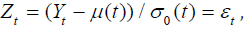, is obtained on the basis of analysis [32] of the sample stationary sequence

For this, statistics are entered

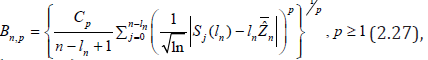
where { , 1} nl n≥ is a sequence of positive integers with 1 n≤ l ≤ n and the notation is entered

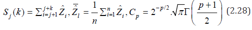
where Γ(•) − is the gamma function? If 0 n l → and / 0 nl n→ as n → ∞ then as , , n p n → ∞ B σ [32]. So, the estimate ˆw σ in (2.26) for sufficiently large n (large T) can be taken as , ˆw n p σ = B (in the calculations, p=1 with c c1= Г(1) and ln( ) nl = n were taken.

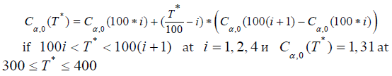
The critical values Cα,0(T*) of statistics (2.25) for different T*= t₂ - t₁ + 1 are defined in [23]. At a level of significance α =0.05, the asymptotic (for large T *) values of Cα,0(T*) in [23] are determined to be 1.27; 1.30; 1.31; 1.33; 1.358 at Т*=100; 200; 300; 400; 500; ∞ respectively. Linear interpolation for intermediate T* values gives the following values

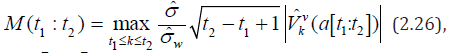
From (2.7), (2.10), (2.16), taking into account the estimate ˆσ = S_T / T , the statistics (2.26) with ν=0 can be written as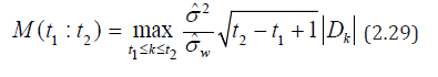

Therefore, the critical values of the statistics (2.26) with ν=0 are written as

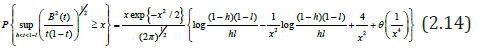
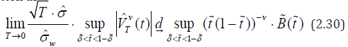
To determine the critical values of the statistics (2.26) with ν=1/2, you can use the asymptotic relation (2.13), written as

Solve x nonlinear equation

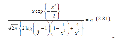
obtained from the curve of part (2.14) with h = l = δ . Under the initial condition x=x0 (for example, x0=100) we find the solution x* of equation (2.31) for fixed α in the MATLAB system. Then the value 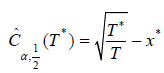can be taken as the critical value of the statistics (2.26) with v = 1 2 .

Modified Method for Predicting the Status of the Cardiovascular Systems on the Basis of Identifying the Boundaries of Quasistationary Sections of The Time Series

To solve the problem of predicting complex digital signals, it was proposed in [17] to use the last “stable” fragment of a time series for training a predictor, obtained by dividing into quasi-stationary regions. Such a task is known [33,34] as a problem of detecting a “debugging”, i.e. changes in the probability properties of the signal. Such a definition can give for complex signals an inaccurate border of a true change in the dynamics of a signal. To detect the change in the dynamics of a complex signal, it was proposed to use an estimate of the local fractal dimension based on the fractality index μ of the time series [19].

As shown in section 1, it is most appropriate to characterize the non-stationary time series with two indicators b(t) and μ(t) included in the power representation (1.14) of the amplitude variation ( ) f V δ of the function f(t) graph corresponding to the original time series. In this case, the value of b(t) is closely related to the volatility (conditional variation) of the time series, according to a jump in which in [18] an algorithm for segmentation of a nonstationary time series was developed.

Given this property of the function b(t), we can propose the following method for detecting the boundaries of quasistationary portions of the time series. Using the sliding window’s original signal f(t), the derived estimation signal b(t), which characterizes the local fractal dimension of the time series, is plotted. In the derivative and in the original signal according to the algorithm [18] are the points of disorder. The positions of these points are compared and the average is taken, which will be the boundary of the adjacent quasi-stationary areas. The fragment of the last generated quasi-stable signal dynamics is used as a learning set for the predictor.

To increase the efficiency of the Q-event forecast, i.e. a record of the rhythmogram of a heartbeat, a larger threshold Q, in the selected last quasi-stationary segment of the time series of the rhythmogram, a combination of the algorithm of repeated intervals using long-term memory [6] with the method of reaching the threshold of change [16] is used.

The RIA approach is based on the analysis of the nonlinear component of the long-term dependence of repeated intervals rj between events xi exceeding a certain defined threshold Q (Q-events).

Sometimes, instead of the threshold K, the average repeat interval or repetition period is set to 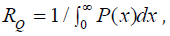where P(x) is the distribution of events { } i x .

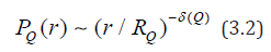
In this approach, to predict random signals with fractal properties, the mathematical apparatus of interval statistics is used when the probability WQ (t;Δt) that during the time Δt appears at least one Q-interval if during the time t for the last Q- event Q event has occurred.

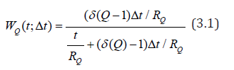
where ∂(Q) characterizes the density distribution of the lengths r of repeated intervals

The method of reaching the threshold of change is based on the transformation of the original signal into a series of times to reach the threshold P:

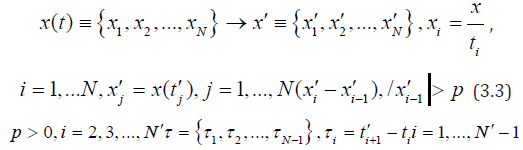
where N is the number of samples in the original signal, x′ is the converted signal, where only those values are left, the relative difference between which exceeds a certain predetermined threshold p, N′ is the number of samples in the converted signal, τ-time series to reach the threshold of change p, where each value of τ-means the time it took the signal to exceed the threshold of change p. The coincidence of the signs of differences x_i′ −x_i-1 ′ and (τ_i − τ_i-1) indicates the persistence (steady growth) of both the values x′_i and the time τ_i between records x_i′ and x_i-1′ . In application to records (extreme events) heartbeat means records and steady increase of intervals between consecutive records. Under the records of the heartbeat can be understood Q-events, and the intervals-Q intervals. Transformation (3.3) can be used to pre-select heartbeat records in the Q-interval prediction procedure, based on the RİA technique, which allows speeding up the last procedure and increasing the reliability of the prediction obtained.

References

• Bunde A, Eichner JF, Havlin S, Kantelhard JW (2003) The effect of long correlation on the return periods of rare events. Physica A 330: 1-7.
• Bogachev MI, Eichner JF, Bunde A (2007) Effect of Nonlinear Correlations on the Statistic of Renturn Intervals in Multifractal Date Sets. Physical Review Letters 99(24): 240601.
• Hllirberg S, Altmann EG, Holstein D, Kantz H (2007) Precursors of ectreme increments. Phys Rev E 75: 016706.
• Bogachev MI, Eichner JF, Bunde A (2008) The effects of multifractality on the statistics of return intervals. The European Physical Journal Special Topics 161: 181-193.
• Bogachev MI, Eichner JF, Bunde A (2008) On the Occurrence of Extreme Events in Long-term Correlated and Multifractal Data Sets. Pure appl Geophys 165: 1195-1207.
• Bogachev MI, Kireenkov I, Nifontov E, Bunde A (2009) Statistics of return intervals between long heartbeat intervals and their usability for online prediction of disorders. New Journal of Physics 11: 063036.
• Bogachev MI (2009) On the issue and predictability of emissions of dynamic series with fractal properties when using information about the linear and non-linear components of the long-term dependence. News Universities of Russia, Radio electronics, 5b: 31-40.
• Bogachev MI (2010) Comparative analysis of the noise immunity of methods for predicting emissions of random signals with fractal properties using information about short-term and long-term dependencies. New Universities of Russia, Radio electronics, 1: 11-21.
• Bogachev MI, Bunde A (2011) On the predictability of extreme events in records with linear and nonlinear long-range memory: Efficiency and noise robustness. Physical A 390: 2240-2250.
• Ludescher J, Bogachev MI, Cantelhard JW, Schumann A, Bunde A (2011) On spurious and corrupted multifractality: The effect of additive noise, shorm-term memory and periodic trends. Physica A 390: 2480-2490.
• Abdullaev NT, Dyshin OA, Ibragimova IJ (2016) The effectiveness of the use of long-term correlations in the differential diagnosis of cardiacvascular system. Biotechnosfera 5: 27-33.
• Abdullaev NT, Dyshin OA, Ibragimova IJ (2018) Comparative analysis of emission prediction methods in the dynamics of the heartbeat in the presence of additive random interference. Proceedings of the XIII International Scientific Conference FREME-2018. Vladimir-Suzdal, Book 1, p. 169-173
• Abdullaev NT, Dyshin OA, Ibragimova IJ (2018) Prediction of emissions of time series with fractal properties of heartbeat intervals. Proceedings of the XIII International Scientific Conference FREME-2018. Vladimir- Suzdal, Book 1, p. 173-177.
• Abdullaev NT, Dyshin OA, Ibragimova IJ (2016) Diagnosis of Heart Diseases Based on the Repeat Interval Statistics of Extreme Events of Heart Rate, Trudy FREME. Vladimir 1: S.43-46
• Abdullayev NT, Dyshin OA, Ibragimova ID (2017) Prediction of the cardiovascular System on the assessment of Repeated Extreme Values Heartbeat Intervals and Times to Achieve Them in the Light of shortterm and long-term Relationships. Journal of Biomedical Engineering and Medical Devices USA, Canada, Europe, Great Britain, 2(2): 1000126
• Yegoshin AV (2007) Analysis of the time the signal reaches the threshold of change in the task neural network time series forecasting. Informationcomputational technologies and their applications. Collection of articles of the VI International Scientific and Technical Conference.: RIO PGSA, Penza, p.74-76.
• Sidorkina IG, Egoshin FV, Shumnev DS, Kudrin PA (2010) Prediction of complex signals based on the selection of the boundaries of implementations of dynamic systems. Scientific and Technical Bulletin of the St. Petersburg State University of Information Technologies, Mechanics and Optics, 2(66): 49-53.
• Abdullaev NT, Dyshin OA, Ibragimova ID, Akhmedova Kh R (2019) Segmentation of non-stationary physiological signals with fractal properties. Information Technologies 5: 300-312.
• Starchenko NV (2005) Fractality index and local analysis of chaotic time series Dis. Candidate of Physics and Mathematics, Moscow, MEPI, pp. 119.
• Kronover RM (2000) Fractals and chaos in dynamic systems. Postmarket, pp. 350.
• Feder E (1991) Fractals. Mir pp. 374.
• Mantegna RN, Stanley G Yu (2009) Introduction to econophysics. Correlations and complexity in finance. Pers eng, Book House, Librocom, pp. 192.
• Inclan C, Tao G (1994) Use of Cumulative Sums of Square for retrospective detection of changes of varicence. Journal of American Statistical Association 89(427): 913-923.
• Krishnaiah P, Miao B (1988) Revive about estimation of chance-points. Handbook of Statistics 7: 375-402.
• (1994) Change-point problems. Lecture notes and monograph series. E Carlstein, HG Muller, D-Siegmunal (Eds.), Institute of Mathematical Statistics, Hargward, CA, Canada, 23: 385.
• Mandelbrot BB (1982) The Fractal Geometry of Nature. WH Freeman, Sun-Francisco, pp. 468.
• Chen G, Choi Y, Zhou Y (2005) Nonparametric estimation of structural change points in volatility models for time series. Journal of Econometries 126(1): 79-114.
• Csorgo M, Horvath L (1997) Limit theorems in chance-point analysis. Wiley, New York pp. 438.
• Xia Y, Tong H, Li WK (1988) Abstitude deviation estimation of volatility in nonparametric models. Research report No.177, Department of statistics and actuarial sciences the University Hong Kong, Hong Kong, pp.133-178.
• Choin JM, Muler HG (1999) Nonparametric quasilikelihood. The annual of statistics 27: 36-64.
• Smolentsev NK (2008) Fundamentals of the theory of wavelets. Wavelets in MATLAB, DMK Press, pp. 448.
• Peligrad M, Shao QM (1995) Estimation of the variance of partial sums for ρ- mixing random variables. Journal of multivariate analysis 52: 140- 157.
• Shiryaev AN (1976) Statistical sequential analysis. Science pp. 272.
• Darkhovski BS (1994) Nonparametric methods in change-point problems a general approach and some concrete algorithms. IMS Lecture Notes-Monograph Series (23): 99-107.