An Exploratory Study Assessing Data Synchronising Methods to Develop Machine Learning-Based Prediction Models: Application to Multimorbidity Among Endometriosis Women

Introduction

Data science is a rapidly evolving research field that influences analytics, research methods, clinical practice and policies. Access to comprehensive real-world data and gathering life-course research data are primary challenges observed in many disease areas. Existing real-world data can be a rich source of information required to better characterise diseases, cohort specification and clinical gaps to conduct more precision research that is value based to healthcare systems. A common challenge linked to real-world and research data is a high rate of missingness. Historically, statistical methods where possible were used to address missing data but advances in artificial intelligence techniques has provided improved methods for use. These methods could also be used for predicting disease outcomes, diagnostic accuracy and treatment suitability.

These methods can be useful for women’s health conditions, where the complex physical and mental health symptoms can give rise to insufficient understanding of disease pathophysiology and phenotype characteristics that play a vital role in diagnosis, treatment adherence and prevention of secondary or tertiary conditions. One such condition is Endometriosis. Endometriosis is a complex condition with an array of physical and psychological symptomatologies, often leading to multimorbidity [1]. Multimorbidity is considered as the co-existence of 2 or more conditions in any given individual and therefore could be prevented if the initial conditions are managed more effectively [2]. The incidence of multimorbidity has increased with a rising ageing population, burden of non-communicable diseases in general and mental ill health. A key feature of multimorbidity is disease sequalae where a physical manifestation could correlate with a mental health impact, and vice versa [1,3]. The precise causation is complex to assess due to limitations in the current understanding of disease sequalae pathophysiology. As such, multimorbidity could be deemed as highly heterogeneous [1-3]. Multimorbidity impact people of all ages, although current evidence suggests it is more common among women than men although previously, multimorbidity was thought to have been more common in older adult that had a high frailty index score [3,4]. Hence, multimorbidity is challenging to treat, and there remains a paucity of research available to better understand the basic science behind the complex mechanisms that could enable better diagnosis and management long-term [5-8].

This undercurrent of disease complexities linked to endometriosis that could lead to multimorbidity should be explored to support clinicians and healthcare organisations to future proof patient care. In line with this, exploring a new method that could demonstrate better predictions and using a new solution to sample size challenges.

Methods

Our primary aim of the study is to develop an exploratory machine learning model that can predict multimorbidity among endometriosis women using real-world and synthetic data. To develop these models existing data with various symptoms and commodities as well as other characteristics were used. Anonymised data were provided by the Manchester and Liverpool Endometriosis specialists centres in the UK. The data record used included symptoms, diseases, and conditions in women with a confirmed diagnosis of endometriosis. Data curation was completed for the entire sample size.

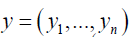
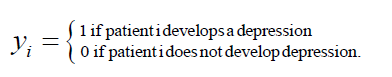
The model used age, height, symptoms, commodities and weight in a mathematical formulation. Let x_i be the vector containing these recordings for the i^th person and let be the matrix containing the data about all n people. As part of developing methodological rigour, we considered a working example was used to predict whether each person in the sample develops depression. Let be the vector of response variables where

Suppose we collect data for n=3 people, as summarised in Table 1. In this example, we have collected p=3 recordings for each person i, these include their age, height and weight, represented by and respectively (Table 1).

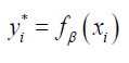
We produced a function, f_β with parameters β, that, for person i, takes as input their age, height and weight and outputs a prediction of whether they will develop depression. Let y_i∗ be the prediction of whether person  develops depression, then we say that

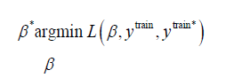
The performance of parameters β acan be tested through a loss function, defined as L(β) which measures the difference between the true values of y and the predictions, . The loss function imposes a penalty when incorrect predictions are made. Hence, to find the best β, we solve the optimisation problem

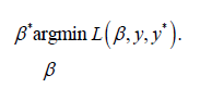
Table 1: Example Dataset for Predicting Depression.

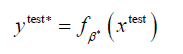
The function f_β can then be used to make predictions for patients who haven’t been tested for depression.

An initial observation was that our prediction function could become over-fitted to the data. This meant that the function captured the specific distribution between x and y very well, but if this data was not in a structured format of the true distribution between symptoms and comorbidities, the prediction function would not be generalisable to other types of data.

The performance of the prediction function on unseen data can be estimated by separating the data into a training set, and test set, 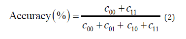. The optimal parameters are found using the training set and then the model’s accuracy is tested on the test set. This accuracy is measured by the proportion of correctly classified data. This is measured by a confusion matrix, which records the frequencies of each possible outcome. Let c be the confusion matrix defined as

where C_ij is the number of times . The accuracy of our model is then

To summarise, the approach is broken down into the following three steps,

1. Solve optimisation problem

on the training set, where the set of prediction values, y^train*, is found by

2. Make predictions on the test set using optimal weights β^*

3. Construct confusion matrix, C as is defined in (1) and find the accuracy of the model on unseen data by equation (2).

Data Preparation-Manchester

In the Manchester dataset, for each patient, the presence of various symptoms and multiple diagnoses among women with Endometriosis. These are summarised, with descriptions in Table 2. A total of p =15 recordings are made for each person and so we define 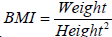to be the vector containing the recordings for person i (Table 2).

Table 2: Manchester Data Feature Variables.

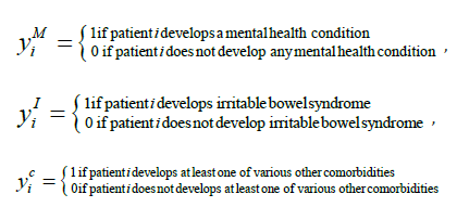
Also for each person, three response variables are recorded, these are summarised, with descriptions, in table 3. These variables are defined as

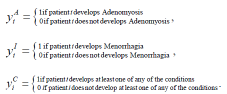
(Table 3).

Table 3: Manchester Data Response Variables.

We examined three models of fit, one for each response variable. We defined a fourth response variable, “Combined”, as shown in the final row of Table 3, which indicates the presence of at least one of the other three conditions. Formally, y_Comb is defined as

We fitted a fourth model for this response variable.

We converted the binary variables, including our response variables of “Yes” and “No” to 1 and 0, respectively. There was no missing data in the Manchester dataset and as such we make use of all n = 99 observations.

Data Preparation-Liverpool

The data from Liverpool, had a sample size compromised of anonymous 913 patients. The raw data defined 68 possible different feature variables for recordings of various diseases and symptoms of each patient. We found a lot of missing data from numerous features. The complete list of features along with their percentage missing values can be found in Table 4.

Table 4: Liverpool Data Percentage Missing Data.

To prepare the data, we filtered by “Endometriosis = TRUE”, to find only those patients who have already been diagnosed with Endometriosis, leaving us with 339 patients. Next, we removed all features with more than 1% of missing values which leaves us with 29 features. However, the first of these, “Sample ID” is simply a unique identifier and is also dropped from the data. The feature “Endometriosis” is a binary identifier, which after filtering, is always true, so we drop this feature too. The final 27 features are summarised, with descriptions, in Table 5 (Table 4,5).

Table 5: Liverpool Data Features with Less than 1% Missing Data.

We found a total of 4 patients now containing missing values and dropped these from the data too, leaving us with patients. We selected two diseases to be our response variables that we will attempt to predict, these response variables are summarised in Table 6. Since we were ultimately interested in predicting multimorbidity in patients, we constructed a final response variable, “Combined”, a binary variable to represent the presence of at least one of the other two response variables, similarly to the data from Manchester. Their formal definitions are

(Table 6)

Table 6: Liverpool Data – Response Variables.

Synthetic Data

It is sometimes the case that real data comes with issues of confidentiality. Especially in medical research, data are likely to contain private and sensitive information which becomes vulnerable when the data are shared for analysis. We used the Synthetic Data Vault (SDV) package in python to develop the synthetic data as a replacement and tested its similarity to the real data. Through the use of other sampling techniques, such as random simulation, the synthetic data could produce a dataset with an advanced sample size that would better represent the whole population.

When preparing our data, we removed many observations due to missing data. Such data could be replaced by generating a synthetic replacement. For our analysis, we instead generated all new observations, rather than filling in missing gaps.

We used SDV’s Gaussian Copula model, a distribution over the unit cube [0.1]^Ρ is constructed from a multivariate normal distribution over R^Ρ by using the probability integral transform. The Gaussian Copula describes the joint distribution of the random variables representing each feature by analysing the dependencies between their marginal distributions. Once fitted to our data, we can use the model to sample more instances of data.

Manchester Data

We began with the Manchester data, after fitting the Gaussian Copula to our 99 samples, we generated 1000 more. Using SDV’s SD Metrics library we can evaluate the similarity between the real and synthetic data. We assessed how closely it relates to the real data to determine whether we have sufficiently captured the true distribution. We did this by comparing the similarity of the distribution over each feature and we took two approaches to assess this similarity.

Initially we measured the similarities across each of the features by way of a comparison of the shape of their frequency plots as demonstrated in Figure 1. This comparison was conducted based on the distribution over “age” for the real and synthetic data (Figure 1).

Figure 1: Age distribution Shape Comparison.

For numerical data, SDV calculated the Kolmogorov-Smirnov (KS) statistic, which is the maximum difference between the cumulative distribution functions. The value of this distance is between 0 and 1 where SDV converted to a score by

Score =1-KS-statistic

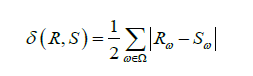
For Boolean data, SDV indicates the Total Variation Distance (TVD) between the real and synthetic data. We identified the frequency of each category value and expressed this as a probability. The TVD statistic compared the differences in probabilities, given by

where Ω is the set of possible categories and R_ω and S_ω are the frequencies of category ω in the real and synthetic dataset respectively. The similarity score is then given by

The score for each feature is summarised in Figure 2, we found an average similarity score of 0.92 (Figure 2).

Figure 2: Feature Distribution Shape Comparison.

For the second measure of similarity, we constructed a heatmap to compare the distribution across all possible combinations of categorical data. This was achieved by calculating a score for each combination of categories. To begin finding these scores, we constructed two normalised contingency tables, one for the real data and one for the synthetic data. Let α and β be two features, the contingency tables describe the proportion of rows that have each combination of categories in α and β, this describes joint distributions of these categories across the two datasets.

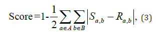
To compare the distributions, SDV calculated the difference between the contingency tables using Total Variation Distance. This distance is then subtracted from 1, meaning that a higher score indicates a higher similarity. Let A and B be the set of categories in features α and β respectively, the score between features α and β are calculated as

where S_a,b and R_a,b are the proportions of categories a and b occurring at the same time, taken from the contingency tables, for the synthetic and real data respectively. Note here that we did not make use of a measure of association between features, such as Cramer’s V, since this does not measure the direction of the bias and so can lead to misleading results.

A score of 1 indicates that the contingency table was exactly the same between the two datasets, and a score of 0 shows that the two datasets were as different as they can possibly be. These scores for all combinations of features are plotted as a heatmap in Figure 3. Note here that continuous features, such as “Age”, were discretized in order to use equation (3) to find a score. The heatmap suggested that most features are distributed very similarly across the two datasets with an exception for “Year of Diagnosis”. Perhaps this could be because of the nature of this feature being a date, yet it was being treated as an integer in the model. This could be an area for further investigation.

From these metrics, we concluded, with confidence, that the new data followed a very similar distribution to the old data (Figure 3).

Figure 3: Distribution Comparison Heatmap.

Liverpool Data

To generate synthetic data, we followed the same procedure as with the Manchester data. We generated 1000 more samples from a gaussian copula fitted to the 311 real samples and combined them with the real data to produce a new dataset. From contingency tables we produced a heatmap using the formula in equation (3) to generate scores, this heatmap can be found in Figure 4. A score of 1 indicates that the contingency table was exactly the same between the two datasets, and a score of 0 shows that the two datasets were as different as they can possibly be. We saw from our plot that we got an average similarity of 0.94 (Figure 4).

Figure 4: Real Vs Synthetic Data Distribution Heatmap (Liverpool Data).

The shape of the distributions were compared for each feature, as an example, the distributions for feature “Height” are plotted in Figure 5. We saw that the distributions are not similar. We used the KS statistic for numerical features and Total Variation Distance for Boolean features to compute similarity scores. These scores are summarised in Figure 6. We saw that the distributions of “Height” and “Weight” were not similar, however, the distributions of the remaining features were similar. We got an average similarity of 0.75 and we concluded that, on average, the distributions of the data were similar. The distributions of all categorical features were captured well, however, two of the continuous features were not (Figures 5,6).

Figure 5: Height Distribution Shape Comparison (Liverpool).

Figure 6: Feature Distribution Shape Comparison Between Real and Synthetic Data (Liverpool).

Models

We considered three standard classification models to predict the response variables; Logistic Regression (LR), Support Vector Machines (SVM) and Random Forest (RF) since they approach separating the data in different ways and offer different insights.

Logistic regression allowed us to find the likelihood of each class occurring. It offers easy interpretability of the coefficients of the model; we can perform statistical tests on these coefficients to interpret which features have significant impact on the value of the response variable. While logistic regression takes a more statistical approach, maximising the conditional likelihood of the training data, SVMs take a more geometric approach, maximising the distance between the hyperplanes that separate the data. We fitted both logistic regression and SVMs in order to compare the performance of these approaches.

While SVMs and logistic regression attempt to separate the data with a single decision boundary, random forest make use of decision trees which bisect the decision space into small regions by use of multiple decision boundaries. These approaches perform differently depending on the nature of the separability of the data. As such, we fitted all three and compared their accuracies to assess the useability of the synthetic data.

Logistic Regression

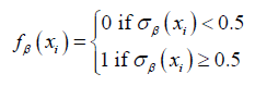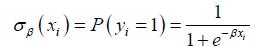
Let to be the general vector of response variables and let be the corresponding vector of features for patient i. We defined the function

to be the probability of patient i developing the condition corresponding to y, where 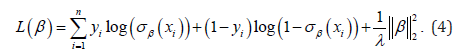are some weights. The prediction function is then defined to be

We found the optimal weights by solving the optimisation problem

where, for logistic regression, the loss function L took the form

Finally, we added regularisor terms λ to avoid overfitting which assisted with capturing the underlying distribution of the data, without the proposed model becoming too specific to the data it was trained on. This helped prevent any potential biases.

SVMs

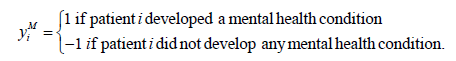
Then we considered Support Vector Machines. We slightly redefined our response variables from binary {0,1} to binary {-1,1}. For example, suppose  would be the binary response for a patient developing a mental health condition, then  is defined as

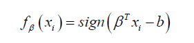
For SVMs, the prediction function takes the form

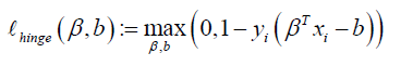
Where and are some weights. We considered the hinge loss function, defined as

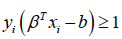
The function is 0 when , which occurs when 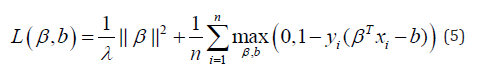or in other words, when we have made a correct prediction. Conversely, when 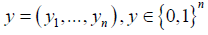, we would incur some penalty. Hence, for SVMs, the loss function, L takes the form

where λ is a parameter controlling the impact the of regularisation term. Similar to logistic regression, this term controls a trade-off between capturing the distribution of the whole population and overfitting to the training data.

Random Forest

The final model we fitted is the random forest predictor. These random forests classified data points through an ensemble of decision trees. The decision trees worked by separating the predictor space by a series of linear boundaries. As before, we let be our set of response variables with corresponding feature vectors where each To build our random forest we followed the procedure,

For b =1,..., B :

Sample, with replacement, and from from x and y respectively.

Fit k decision trees, to dataset

When making predictions on unseen data, the model took the majority vote across all trees.

For all experiments, we split the real data in half, giving us one training set of real data and one test set of real data. The whole synthetic data is used as training data. All models used the test set of real data, thus allowing us to compare the performance between models trained on real data and models trained on synthetic data.

Results

For all experiments, we trained one model on real data, and one on synthetic data. Both are tested on the same test set which contains only real data, because we can be sure that the real data are drawn from the overall population’s true distribution. The accuracies of these models can then give us insight into whether the use of synthetic data affects the performance of machine learning models.

All the models contain hyperparameters that impact the performance of the model on unseen data. For each model, we perform hyperparameter optimisation by a grid search, measuring the accuracy by cross-validation, to find the optimal selection of the hyperparameter. k -fold Cross-validation separates the data into k subsets, and by training the model on k-1 subsets and testing on the remaining set, we get an estimate of how the model will perform on unseen data. This process is repeated, holding out a different subset for testing each time, and an average performance is taken. We perform cross-validation grid search using the training data and select the value of the hyperparameter that gives the best average accuracy and then retrain the model on the complete training set.

Manchester Data

We divided the real-world data into a training set of 50 samples and a test set of 49 samples. The synthetic data remains as a training set of 1000 samples.

Logistic Regression

We used scikit learn to fit logistic regression models of the form in equation (4). We performed a grid search using 5-fold Cross-Validation (CV) to investigate the optimal value of λ. The CV accuracies for each response variable can be found in Figure 7. For each response variable, the λ that gave the highest CV accuracy is chosen, refitted to the whole training set and tested on the test set. The accuracies on the test set and summarised in Table 7 (Figure 7) (Table 7).

Figure 7: Age distribution Shape Comparison.

Table 7: Logistic Regression Cross-Validation.

We can see that for all response variables, the models performed slightly better when trained on synthetic data.

SVM

We used Scikit Learn’s svm.SVC to train and test SVMs of the form in equation (5) on our data, Scikit Learn is a popular and well-tested choice for SVMs that has shown high performance on a variety of types of datasets. We performed a grid search using 5-fold cross validation to find the optimal value of , these are summarised in Figure 8. For each response variable, the  that gave the highest CV accuracy is chosen, refitted to the whole training set and tested on the test set. The accuracies on the test set are summarised in Table 8. We can see that the models trained on synthetic data performed the same as the models trained on real data for all response variables except “Comorbidities (other)” where the model trained on synthetic data performed better, giving the models trained on synthetic data a better performance on average (Figure 8) (Table 8).

Figure 8: SVM Cross-Validation.

Table 8: SVM comparison with synthetic data.

Random Forest

Finally, we fitted random forest models to the data. For each response variable, we used 1,5,10,…,500 trees, and performed a grid search using 5-fold cross-validation to find the best number of trees. The CV accuracies are summarised in Table 9. For each response variable, the number of trees that gave the highest CV accuracy is chosen, refitted to the whole training set and tested on the test set. The accuracies on the test set and summarised in Table 9 (Figure 9) (Table 9).

Figure 9: SVM Comparison with Synthetic Data.

Table 9: Random Forest Comparison with Synthetic Data.

We can see that the models trained on synthetic data performed better than the models trained on real data for all response variables

Solver Comparison

To summarise, the average accuracies of all four models are summarised in Table 10. We can see that, on average, the models trained on synthetic data performed better than the ones trained on real data, supporting the use of synthetic data as a replacement to real data (Table 10).

Figure 10: Age distribution Shape Comparison.

Table 10: Sensitivity Analysis on Manchester Data.

Sensitivity Analysis

To test the sensitivity of our models we added random noise to the data and measured how much this affected the accuracy of the models. Sampling from a unform distribution, we randomly selected 1% of points in each dataset to add noise to. The values at these points were replaced by randomly sampling from a uniform distribution over the feature’s possible values. Table 11 summarises the accuracy of the new models as well as their relative percentage change in accuracy (Table 11).

Table 11: Comparison of all Models.

We can see from Table 11 that the accuracy of the model was affected in some cases. The logistic regression model trained on real data was affected by more than 2% while the accuracy of its synthetically trained counterpart was only changed by 0.5%. Neither dataset shows a consistency to how the models were affected.

Liverpool Results

We divided the real-world data into a training set of 154 samples and a test set of 154 samples. The synthetic data remains as a training set of 1000 samples.

Logistic Regression

We used scikit learn to fit logistic regression models of the form in equation (45) and performed a grid search using 5-fold cross-validation to investigate the optimal value of λ . The CV accuracies for each response variable can be found in Figure 10. For each response variable, the λ that gave the highest CV accuracy is chosen, refitted to the whole training set and tested on the test set. The accuracies on the test set and summarised in Table 12 (Figure 10) (Table 12).

Figure 10: Logistic Regression Cross-Validation.

Table 12: Logisitc Regression Model Comparison (Liverpool).

The models (Table 12) trained on synthetic data performed the same for predicting adenomyosis and better for the remaining response variables

SVM

We used Scikit Learn’s svm. SVC to train and test SVMs of the form in equation (5) on our data, and performed a grid search using 5-fold cross validation to find the optimal value of λ , these are summarised in Figure 11. For each response variable, the λ that gave the highest CV accuracy is chosen, refitted to the whole training set and tested on the test set. The accuracies on the test set and summarised in Table 13 (Figure 11) (Table 13).

Figure 11: SVM Cross-Validation.

Table 13: SVM Model Comparison.

The models trained on synthetic data performed better for all response variables (Table 13).

Random Forest

We fitted random forest and performed a grid search using 5-fold cross-validation to test 1,5,10,…,500 trees showed a higher degree of CV accuracy (Figure 12). For each response variable, the number of trees that gave the highest CV accuracy is chosen, refitted to the whole training set and tested on the test set. The accuracies on the test set and summarised in Table 14 (Figure 12) (Table 14).

Figure 12: Random Forest Cross-Validation.

Table 14: Random Forest Model Comparison.

The model trained on synthetic data performed the same as the model on for adenomyosis and better for the remaining response variables. Therefore, on average, the models trained on synthetic data performed better.

Solver Comparison

To summarise, all four model’s average accuracies are summarised in Table 15. We saw that the best over-all performing model is the random forest, trained on the synthetic data. We can also see that, on average, the models trained on synthetic data performed better than the ones trained on real data. These results support the use of synthetic data in place of the real data (Table 15).

Table 15: Comparison of all Models.

Sensitivity Analysis

To test the sensitivity of our models we added random noise to the data and measured how much this affected the accuracy of the models. Sampling from a unform distribution, we randomly selected 1% of points in each dataset to add noise to. The values at these points were replaced by randomly sampling from a uniform distribution over the feature’s possible values. Table 16 summarises the accuracy of the new models as well as their relative percentage change in accuracy (Table 16).

Table 16: Sensitivity Analysis on Liverpool Data.

We can see from Table 16 that there was little change to the performance of the models for logistic regression and SVM. However, the random forest models saw a significant drop in performance, suggesting that these models are sensitive to perturbations in the data. This could suggest that for the random forest models, it is crucial that the distribution of the synthetic data is highly similar to the real data since the model is sensitive to small changes.

Comparison Across Datasets

(Table 17) Table 17 compares the model accuracies across both datasets. We can see that the models trained on the Liverpool data consistently out-perform the models trained on the Manchester data, for both real and synthetic data.

Table 17: Comparison of all Models.

The two datasets recorded different attributes of the people, as well as containing differing numbers of features and observations. The Liverpool dataset saw a larger number of both features and observations, and we saw our method perform well in both datasets. These results help to support the idea that our method can be applied to a variety of datasets. The experiments have also shown how effective our method is with both continuous and categorical data. We saw from the distribution analysis of the Liverpool synthetic data, that our method performed at its worse on two continuous features.

In the experiments, we have demonstrated that the models trained on synthetic data performed similar or better than the ones trained on real data. Since all models were tested on real data, we can use this to support the argument that synthetic data can be used as a replacement of real data.

Discussion

Multimorbidity is a cause for concern within a growing global population. It is a significant concern for those with chronic conditions such as endometriosis where treatment options are highly limited4. Our results indicate that machine learning can be a useful method to predict the incidence of multimorbidity among endometriosis women who are at a higher risk of developing comorbidities despite the lack of emphasis this in the clinical domain at present. These findings emphasise that the method could be replicated to other complex women’s health conditions such as polycystic ovary syndrome.

These findings indicated that the real-world dataset comprised of one variable to be a significant indicator for developing multimorbidity and the usefulness of synthetic data for future research, especially where there is a higher rate of missing data5. Synthetic data can also show more detailed information in regard to the correlator relationships between these variables as they could be considered as significant indicators. These indicators can be used to differentiate between samples that may have symptoms versus those with a disease sequalae that would influence the clinical decision-making process especially for those requiring excision surgery.

With an advanced sample size and better representation of the overall population, synthetic data has the potential give us more detailed information about the significance of each feature. These indicators can be used to differentiate between samples that may have symptoms versus those with a disease sequalae that would influence the clinical decision-making process especially for those requiring excision surgery.

The distribution of the synthetic data captures the true distribution of the real-world data but the former can have an arbitrary larger sample size, indicating that synthetic data has the potential to provide insightful information for healthcare services in particular. To meet the increasing and complex healthcare demands of a growing population, clinical service design is vital for sustainability of healthcare. Furthermore, the results show that the synthetic data accurately represents the real data and so can be used in place of the real data in cases where the real data contains sensitive or private information that cannot be shared. The accuracy measures of our models support the idea that the use of synthetic data does not affect the performance of the prediction models used in this analysis.

Limitations

The model performance will require to be tested on more complex and large data-sets to ensure a digital clinical trial can be conducted to optimise the model performance.

Conclusion

Prior to experimenting the models developed with the real-world dataset, a quality assessment test was conducted by comparing the synthetic and real-world datasets. Distribution and similarity plots suggested that the synthetic data did indeed follow the same distribution. Therefore, synthetic data generation shows much promise, especially useful for conducting quality clinical epidemiology and clinical trials that could devise better precision treatments for endometriosis and, possibly prevent multimorbidity.

Declarations

Funding

Conflicts of Interest

PP has received a research grant from Novo Nordisk and other, educational from the Queen Mary University of London, other from John Wiley & Sons, other from Otsuka, outside the submitted work. SR reports other from Janssen, Lundbeck and Otsuka outside the submitted work. All other authors report no conflict of interest. The views expressed are those of the authors and not necessarily those of the NHS, the National Institute for Health Research, the Department of Health and Social Care or the Academic institutions.

Availability of Data and Material

The authors will consider sharing the dataset gathered upon receipt of reasonable requests.

Code Availability

The authors will consider sharing the dataset gathered upon receipt of reasonable requests.

Author Contributions

GD conceptualised and developed the FEINMAN project and wrote the study plan for work package 1. GD, AZ and PP furthered the study protocol. GD developed the method and furthered this with PP, AZ, DB, JQS, HC, DKP and AS. GD, DB and AZ designed and executed the analysis plan. All authors critically appraised, commented and agreed on the final manuscript. All authors approved the final manuscript.

References

• Delanerolle G, Ramakrishnan R, Hapangama D, Zeng Y, Shetty A, et al. (2021) A systematic review and meta-analysis of the Endometriosis and Mental-Health Sequelae; The ELEMI Project. Womens Health (Lond).
• Alimohammadian M, Majidi A, Yaseri M, Ahmadi B, Islami F, et al. (2017) Multimorbidity as an important issue among women: results of a gender difference investigation in a large population-based cross-sectional study in West Asia. BMJ open 7(5): e013548.
• Tripp Reimer T, Williams JK, Gardner SE, Rakel B, Herr K, et al. (2020) An integrated model of multimorbidity and symptom science. Nursing outlook 68(4): 430-439.
• Oni T, McGrath N, BeLue R, Roderick P, Colagiuri S, et al. (2014) Chronic diseases and multi-morbidity-a conceptual modification to the WHO ICCC model for countries in health transition. BMC public health 14(1): 1-7.
• Delanerolle GK, Shetty S, Raymont V (2021) A perspective: use of machine learning models to predict the risk of multimorbidity. LOJ Medical Sciences 5(5).
• Hassaine A, Salimi Khorshidi G, Canoy D, Rahimi K (2020) Untangling the complexity of multimorbidity with machine learning. Mechanisms of ageing and development 190: 111325.
• Jensen AB, Moseley PL, Oprea TI, Ellesøe SG, Eriksson R, et al. (2014) Temporal disease trajectories condensed from population-wide registry data covering 6.2 million patients. Nature communications 5(1): 4022.
• Giannoula A, Gutierrez Sacristán A, Bravo Á, Sanz F, Furlong LI (2018) Identifying temporal patterns in patient disease trajectories using dynamic time warping: A population-based study. Scientific reports 8(1): 1-4.