Biomechanical Model of Morphogenesis of Spiral Phyllotaxis Patterns and its Computer’s Visualization

Glossary

a) Phyllotaxis (from the Greek phýllon-leaf and taxis-arrangement): covers a very wide range of botanical objects, in the structure of which orderliness, helicity, periodicity or symmetry are observed. These structures, which are often surprisingly beautiful, are usually called phyllotactic patterns.

b) Primordium (plural Primordia): a discrete element (seed germ, seed, leaf, flower petal, new shoot) of a plant.

c) Parastichy (plural Parastichies): visually distinguish­able right- or left-handed spiral formed by primordia.

d) Family of Parastichies: an aggregate of parastichies with the same twist.

e) The Parastichy Index: the number of parastichies in a family. Along with the term “a family of parastichies with index A”, “a parastichy of family A” is also used.

f) The Golden Number (Golden Ratio, Golden Mean): ir­rational number equals to has a large number of unique mathematical properties [1,2,3], in particular τ2 = τ +1.

g) Recurrent Sequence (Recursive Sequence): an integer recurrent sequence whose members are calculated by a recurrent formula:

The most interesting property of recurrent sequence is:

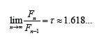
h) The Fibonacci Numbers (The Fibonacci Sequence): a recurrent sequence, with initial terms F₁=1 and F₂=1.

i) Genetic Spiral: an imaginary spiral that sequentially passes through all primordia. In planar phyllotaxy, the genetic spi­ral starts at the center of the inflorescence, while in cylindrical phyl­lotaxy it is the helix.

j) Successive Primordia: two primordia consecutively ly­ing on the genetic spiral/helix.

k) Divergence Angle: the smaller angle between two rays starting at the center of the inflorescence and passing through a pair of successive primordia, respectively. For Fibonacci phyllotax­is, this is the golden angle 2π/τ2.

l) Spiral Phyllotaxis: a specific arrangement of primordia, in which a person sees the right and/or left-handed spirals. It is necessary to distinguish between planar, cylindrical multi-spiral, and cylindrical one-spiral phyllotaxis.

m) Fibonacci Phyllotaxis: pattern of spiral phyllotaxis in which parastichies indices are equal to Fibonacci numbers.

n) Planar Spiral Phyllotaxis: mainly observed on a planar or convex inflorescence. The most striking example of such a phyl­lotaxis is the sunflower inflorescence, on which up to four different families of spirals can be distinguished (Figure 1A).

o) Cylindrical Multi-Spiral Phyllotaxis: mainly observed on cones of various plants. Usually, a human can distinguish be­tween two or three families of parastichies. The most striking ex­amples of such phyllotaxis are pineapple (Figure 1B).

p) Cylindrical Single-Spiral Phyllotaxis: mainly observed on young shoots of various plants. Usually, a person notices that the angle between adjacent primordia is constant and equal to the golden angle 2π/τ2 . You can also mentally draw one spiral through the primordia on young shoots (Figure 1C). The actual index of such phyllotaxis is (1,1).

Figure 1: Spiral phyllotaxis patterns. (A) Planar spiral phyllotaxis at inflorescence of a sunflower with visible parastichies index (21, 34, 55). (B) Cylindrical multi-spiral phyllotaxis at pineapple, index (8, 13, 21). (C) Scheme of cylindrical single-spiral phyllotaxis from [4].

The Phenomenon of Spiral Phyllotaxis

What is the phenomenon of spiral phyllotaxis? First of all, it’s very beautiful! When looking closely, we can see a kind of symme­try, which is not actual symmetry. And when we start counting, we get the Fibonacci numbers and the golden ratio!

Remarkably, we find patterns of spiral phyllotaxis on plants of various species that are far apart in the list of systems of plant tax­onomy. This suggests that quite different plants have a universal morphogenesis of phyllotaxis patterns.

The problem of morphogenesis of phyllotaxis patterns has been of concern for generations of botanists and mathematicians. Thou­sands of measurements have been conducted, hundreds of articles have been written, dozens of books have been published, but there has not yet been a full-fledged theory explaining the morphogene­sis of spiral phyllotaxis. However, numerous studies [5,6,7] provide a sufficient foundation for explaining an objectively existing phe­nomenon. Most researchers note that all types of spiral phyllotaxis are united by the following facts:

a. The number of visible spirals or helix of one family in 96% are Fibonacci numbers, and 3% are other recursive sequences [5,6,7].

b. The ability to mentally conduct a genetic spiral/helix.

c. Divergence angle is constant.

Based on these unifying factors, two main “mysteries” of spiral phyllotaxis morphogenesis were de facto formulated: Why does the number of spirals (parastichies) in each family equal to the mem­bers of the recurrent sequence? And why is the divergence angle equal to irrational number, which contains the golden ratio?

Phyllotaxis in Terms of Philosophy

Before proceeding to the analysis, it is necessary to consider what the objects of study are and answer the question “How does primordium qualitatively differ from the plant on which it ap­pears?” Roots, trunk, branches, and other parts of plants, from the point of view of botany, are a continuous system whereas a primor­dium is always a discrete entity.

If the primordium is a seed, then this difference is even more noticeable, because the essence of a seed is to be separated from the plant and start the growth of a new plant.

The dialectical connection between plant and primordium al­lows us to formulate a philosophical definition of phyllotaxis: Phyl­lotaxis is the process of the emergence of the discrete from the con­tinuous.

Phyllotactic Patterns as Visual Effect

Before starting a quantitative analysis, it is necessary to answer the question: what do we actually see when looking at the phyllo­tactic pattern? At first sight, this question seems to be rather sim­ ple, even juvenile, but as it shows later, the formalization of what we see allows the analysis to go further than the solution to the dual mystery of phyllotaxis.

Let’s look at the inflorescence of a sunflower (Figure 1A), which is a classic example of the plant spiral phyllotaxis pattern. The first thing that catches the eye is the right- and left-handed spirals, which are formed by primordia of the inflorescence of a sunflower (in the case of a sunflower, primordium is an achene). When looking at it closer, we can notice the initial and final seeds between which this spiral is visible.

If, as stated above, a seed is a discrete object, then what are the spirals that we see? Our brain, unconsciously, integrates discrete elements into pseudo-objects that look like spirals. The spirals that we see on the phyllotactic pattern exist only in our brain [3,8].

Video 1, https://youtu.be/qUBoRw8LCFw shows the stretching/ compression of a planar representation of the cylindrical phyllo­taxis, in which the primordia “come together” into parastichies (straight lines in this case) and then “disintegrate”. This confirms that these right- and left-tilted straight lines are only the result of the peculiarities of human perception, which combines nearby pri­mordia into “parastichies”. It is important to note that during this stretching/compression, the structure of the phyllotaxis pattern re­mains constant. In [3,8], it is analyzed in detail what structures can have such properties.

The videos for this article were built by the classic animation technique, but instead of hand-drawn pictures, frames were used which were generated (“drawn”) by a C# program in Windows plat­form Console Application. А separate program was written for each video. Usually, each of these programs generate about 1000 frames. MS Movie Maker (or similar) combines these frames as a slideshow into a video. For these projects, the author has set the duration of each frame up to 0.05 - 0.1 seconds. A detailed explanation of the creation of this video is in Appendix A. The most vivid example of such visual effects is the merging of the stars into constellations, which are unified objects only in human perception. Our brain unites stars and galaxies, which for the observer on the Earth, are visually located from each other at a small angular distance into constellations. However, the real linear distances between the stars, in the same constellation, can be hundreds and thousands of light years, but to the terrestrial observer, these stars seem to be “near.”

This allows us to conclude that human perception unites pri­mordia, being at the minimum distance from each other, into spirals (parastichies).

Static Model of Spiral Phyllotaxis

The basis of the static model of spiral phyllotaxis was laid by Bravais and Bravais [9], Adler and, et al., [10]. Braun [11] and Schim­per [12] assumed that one spiral (which is called the genetic spi­ral) can be drawn through all primordia of the phyllotaxis pattern, and the divergence angle is constant. Based on this assumption, the Bravais -Bravais theorem was formulated by Bravais and Bravais, et al., [9] and Jean [6]: if a family of parastichies with index Q is ob­served on a phyllotaxis pattern, then the difference in the numbers of neighboring primordia lying on the same parastichies is equal to Q. It follows from this that human perception combines primordia with numbers …, M-Q, M, M+Q, M+2Q, M+3Q, . into a spiral (Fig­ure 1A). It was also proposed to the Bravais-Bravais to number the primordia according to the distance from the center of the spiral, which made it possible to carry out a numerical analysis of phyllo­taxis patterns.

In [3], it was analytically found how the distance between the centers of neighboring primordia belonging to the parastichy of family Q depends on the primordium number M:

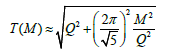
Figure 1A clearly shows more than three parastichies’ families. Let’s assume that three families of parastichies have indices Q, R, S (Q < R < S). Let us construct curves for these parastichies according to the formula above. Each such curve is a graph of the distance be­tween primordia M and M+Q from M for each parastichy (Figure 2).

Figure 2: Graph of the dependence of the distance between neighboring primordia for three families of parastichies have indices Q, R, S.

From the fact that our brain combines nearby objects, it follows that in different areas of the phyllotaxis pattern, we will clearly see that parastichy, the graph of which is below in Figure 2. For exam­ple, for primordia between P and L, we will clearly see parastichies of family R, and in the area of primordia with numbers greater than L, parastichies of family S. The intersection of the curves at the point P means that the distance from the primordium with the number P to the nearest primordia belonging to parastichies Q and R is the same, i.e., in the aria of primordia with numbers close to P, two intersecting parastichies Q and R will be clearly visible. The in­tersection of the curves at point K corresponds to the visual effect, which is known as the ““the phyllotaxis rises” - a visual transition from a pair of parastichies with indices (Q, R) to a pair (R, S).

The range of hypotheses explaining the process of morphogen­esis of phyllotaxis patterns is quite wide. Of those hypotheses that can be recognized as scientifically correct, only two directions can be distinguished: biochemical and biomechanistic.

Why didn’t Alan Turing Solve the Riddle of Phyllotaxis?

As it is known, a plant is a biological object, consisting of many cells, between which various biochemical processes occur. These processes are adequately described by statistical and differen­tial-integral mathematical tools. Therefore, a significant part of researchers tried to build a model of phyllotaxis morphogenesis, relying on mathematical methods that were well tested in biology and chemical.

The most prominent representative of this direction was the outstanding mathematician of our time-Alan Turing, who was one of the fathers of cybernetics. In the early 1950s, Turing published the fundamental article “The Chemical Basis of Morphogenesis” [13] devoted to the self-organization of matter and the self-oscillat­ing chemical reactions. At the same time, Turing was keenly inter­ested in the phenomenon of phyllotaxis and tried to explain it using the same biochemical methods. In 1992, Turing’s unfinished article “Morphogen theory of phyllotaxis” [14] was published, in which he tried to explain the appearance of Fibonacci parastichies by the self-oscillation nature of chemical reactions in plants. However, the Fibonacci numbers do not arise in solving equations describing self-oscillating processes. The Fibonacci numbers also do not ap­pear as basic constants in statistics or in the differential-integral calculus, such as the constant π arises in trigonometry or e in the differential-integral calculus. As stated in [3], recurrent series ap­pear only when solving problems containing recursion. From this, we can assume that the morphology of the spiral phyllotaxis is a recursive process.

Invisible and Visible Primordia

The foundations of the mechanistic approach were laid by the Bravais and Bravais [9], and then continued by Church [5], Mitchin­son [15], Jean [6], Lee and Levitov [17]. It’s also especially necessary to note the research of Adler [18] who formulated the “model of contact pressure”.

At the beginning of the era of mathematical phyllotaxis, Hof­meister [19] postulated that a new primordium was formed far­thest from existing ones. This postulate, known as the “Hofmeister rule”. Moreover, for a flat phyllotaxis (for example, a sunflower, Fig­ure 1A), according to the “Hofmeister rule”, the filling of the pattern with new primordia occurs from the outer edge to the center of the inflorescence, and for a cylindrical (any shoot apical meristem), a new primordium occurs between the vegetative apex and the old primordia.

Let us analyze a typical example of explaining the morphogen­esis of spiral phyllotaxis using the “Hofmeister’s rule”. (Figure 3A) shows a very early stage of the formation of the pattern of phyl­lotaxis in the inflorescence of a sunflower, obtained by a scanning electron microscope from [6] In the center of the inflorescence (a circle with a radius of 2/3 of the radius of the inflorescence), no bulges are noticeable, and in the outer ring with a thickness of 1/3 of the radius of the inflorescence, more than 300 primordia are clearly visible, clearly forming couple parastichies with an index (55, 89). The absence of visible primordia in the center of the in­florescence misled many researchers, for Doudly and Couder [16], Hernandez and Palmer [17] (Figure 3A,3B).

Figure 3: (A) Micrograph taken by J. H. Palmer with a scanning electron microscope from Jean, et al., (1994). Printed with permission from Cambridge University press. (B) The phyllotactic lattice for 2000 elements, obtained similarly to the procedure in Video 2.

Based on the analysis of this micrograph shown above, Jean [6] describes phyllotaxis morphogenesis: “Showing the process of floret initiation proceeding toward the center on the generative front with a remarkable degree of symmetry”. Ibid: “the primordial florets are initiated in rapid succession from the periphery to the center of the apex”; i.e. under the influence of a certain mysterious mechanism, primordia “initiated” from the outer edge to the center, and the divergence angle is maintained with the highest accuracy and the process itself is not subject to probabilistic deviations. This is like the old gunners’ joke: “each bomb always accurately hits the crater prepared for it.”

Despite the obvious fantastic nature, this hypothesis has its merit: primordia, which are located on the periphery of the inflo­rescence, are older than those located closer to the center. The age of primordium is directly proportional to the distance from this pri­mordium to the center of the inflorescence. In [3], it was hypothe­sized that the morphogenesis of the phyllotactic pattern originates from the center of the inflorescence, i.e., each “newborn” primor­dium appears in the center of the inflorescence and in the process of morphogenesis moves to the periphery. So, we can say that the process of morphogenesis consists of two permanent actions:

a) The appearance of a new primordia, in the center of the inflorescence, at regular intervals;

b) Uniform growth of each primordium.

As a result of the growth, each primordium creates pressure on the surrounding primordia. According to the laws of physics, the surrounding primordia create the same pressure on each primordi­um. In [3], it was proved that the resulting vector from the pressure of all primordia on each primordium is directed strictly from the center of the inflorescence. The result of this pressure is the move­ment of each primordium away from the center of the inflorescence.

Just as the birth of a child is a transition from an invisible state to a visible state, primordium, during its growth, also tran­sits from an invisible to a visible state. In [3], the following exper­iment is proposed: let’s take a cup with a flat planar bottom and a set of balls of different diameters and place them in the cup so that each ball would touch the bottom of the cup, then pour an opaque liquid into the cup so that the liquid will cover all the balls. Later on, the liquid will evaporate, and the balls, starting with the largest, will appear above the surface, i.e. become visible Video 2, https://youtu.be/LyHz1bpQ184. Something similar is happening with primordium: while the primordium is very small and located in the receptacle, it is invisible. In the process of growth, the pri­mordium increases and becomes visible, like a tubercle on the re­ceptacle. A detailed explanation of the creation of this video is in Appendix B.

The hypothesis of an invisible and visible stage of development of primordia explains well the features of the phyllotactic pattern on Figure 3B. The primordia located on the periphery are already quite grown and clearly visible, while those in the center are not yet visible, but already exist. If Palmer [17] (which made Micrograph Figure 3A) could use a transmission electron microscope, then we would see primordia inside the receptacle, as in Figure 3B. As noted above, “Nothing is what it seems”, especially when analyzing visual phenomena (Figure 4A,4B).

Figure 4: “Sequential replicas of sunflower meristems after microsurgical manipulation. The same meristem immediately after (A) and three days after (B) performing a centered cut.” - from unpublished results [19]. Published with personal permission from Dr. Dumais.

The hypothesis of the invisible and visible stages of the devel­opment of primordium perfectly explains the phenomenon of cut­ting out a part of the receptacle [17, 19]. Figure 4 clearly shows that cutting out some part of the receptacle does not affect the structure of the rest of the primordia. This clearly indicates that even before cutting, the primordia were already in the receptacle, but still in an invisible stage. This confirms the assumption that each primordium is a separate object, developing according to an autonomous plan, so the removal of a certain number of primordia does not have a significant effect on the growth and location of the other primordia. The second important conclusion from the analysis of these micro­photographs: the formation of the pattern of phyllotaxis takes place during the invisible stage of development of primordia. Therefore, by the time the early primordia on the outer edge of the inflores­cence become visible, the structure of the phyllotactic pattern has been already fully formed.

Solving the First Mystery of Phyllotaxis

Let’s return to the question: “Why is the number of right- and left-handed spirals equal to a pair of neighboring numbers from the recurrent sequence?” Video 2 shows a dynamic model of the de­velopment of spiral phyllotaxis [3,8]. This dynamic model assumes a recursive repetition of the transition from a phyllotaxis pattern with N primordia to a pattern with N+1 primordia, while:

a) Each new primordium is added to the center of the inflo­rescence at regular intervals.

b) Each primordium continuously moves from the center of the inflorescence.

c) Each primordium continuously grows (increases in size).

d) The phyllotaxis pattern keep the genetic spiral and a con­stant angle of divergence.

As can be seen from the above, this dynamic recursive model combines biological growth and mechanical pressure, so for brev­ity we will call it The Biomechanical Model. In contrast to the static model, the numbering of primordia from the center of the inflores­cence in the dynamic model will not be correct. Because the num­bers of primordium, in the static model, is its “age”, and in the bio­mechanical model, “age” changes in time. Therefore, to analyze the change in the location of primordia in the biomechanical model, we will color primordia.

Consider changes in the parastichies of three families Q, R, and S, from the static model above, during recursive growth. On Video 3, https://youtu.be/nqOuWhGp82w, one of the parastichies of the family Q is light blue, R is light red, and S is light green. The primor­dium belonging to all three colored parastichies is colored black, and the three adjacent primordia are blue, red, and green, respec­tively (Figure 5A,5B).

In Figure 5A, the number (age) of the black primordia is P and the blue and the red parastichies are clearly visible. This is the same primordium P and the same parastichies as in Figure 3B. According to the Bravais-Bravais theorem, the age of the blue primordium is Q greater than the black one, and the age of the red one is R greater than the black one.

Accordingly, in Figure 5B, the number (age) of the black pri­mordium is equal to L and the red and green parastichy are clearly visible, it follows that the age of the red primordium is by R more than black one, and the age of green is more by S than black one (Figure 6).

Figure 5: Two frames from Video 3.

Figure 6: The phyllotaxis pattern.

Figure 6 shows a pattern similar to the pattern in Figure 5A. For the simplicity of the explanation, only the centers of primordia were drawn. Let’s formulate the problem: find S if Q and R are known. Let the black primordium, at the moment of time shown in Figure 6, have some number M. Then the blue primordium has the number M+Q (horizontal black arrow), red one has the number M+R, green one has the number M+S. As it can be seen from Figure 6, the blue and green primordia also belong to one of the parastichies of family R (one of the red spirals). This means that the number of the green primordium is R greater than the blue one (vertical black arrow), or equal to M+R+Q. But it was indicated above that the number of the green primordium is M+S, then S=Q+R!

Solving the Second Mystery of Phyllotaxis

Video 4, https://youtu.be/JP0P76RxNps shows a sequence of non-linear 3D transformations over a planar Archimedean spiral. In these transformations, the axis of all solids of revolution coin­cides with the axis that is perpendicular to the plane of the spiral and passing through the center of this spiral. At the beginning of the video, the original planar spiral transforms into a spiral on a hemi­sphere, then a spiral on a cone, then a helix on a cylinder, a helix on a hyperboloid of revolution, and a spiral on a solid of revolution like a pinecone. This shows that a planar spiral can be “stretched” onto any solid of revolution without disturbing the structure of the spiral, if the axes of the spiral and the solid of revolution coincide.

Let us consider one of such 3D transformations over the ge­netic spiral and the primordia “attached” to it. The genetic spiral “stretched” on the cylinder is transformed into a genetic helix, and the primordia visually form a pattern of cylindrical phyllo­taxis. Moreover, if the genetic helix has a small pitch, then this is a multi-spiral pattern, and if the genetic helix is strongly stretched (long pitch), then this is a single-spiral phyllotaxis. This is due to the visual nature of the parastichies, which was shown in Video 1, Vid­eo 5 https://youtu.be/dvvJG6P3K_M shows the morphogenesis of a planar phyllotaxis pattern, transforming it into a multi-spiral cylin­drical pattern, and then stretching it into a single-spiral pattern of phyllotaxis. The second feature of the transformation of a planar phyllotaxis pattern into a cylindrical one is the preservation of the divergence angle unchanged. The persistence of the divergence an­gle between two cyan-colored successive primordia can be seen in Video 5 at all stages of transformation (Figure 7A,7B).

Figure 7: Three frames from Video 5. (A) Planar spiral phyllotaxis. (B) Cylindrical multi-spiral phyllotaxis. (C) Cylindrical single-spiral phyllotaxis.

Also, in Video 5, we can see the similarity between the patterns drawn by the biomechanical model at various stages of transforma­tion and real botanical objects. This is clearly seen when comparing Figure 1 and Figure 7.

Conclusion

In this study, various aspects of phyllotaxis morphogenesis were considered:

Philosophical: Phyllotaxis is the process of the emergence of the discrete from the continuous.

Psychological: the visible spirals on the phyllotaxis pattern are a visual effect, combining discrete objects into a pseudo-object.

Mathematical: Fibonacci numbers appear only when solving problems that contain recursion.

Morphogenetic: forming of phyllotaxis patterns is a biomech­anistic recursive process.

There was proposed the biomechanical model of planar phyl­lotaxis: a new primordium was added to the center of the inflores­cence at regular intervals, and each primordium continuously and

evenly increased in size.

There are two implications of the biomechanical model:

a) The index of the next parastichies family is equal to the sum of the indices of the two previous families.

b) The divergence angle is constant.

A cylindrical phyllotaxis pattern is obtained by stretching a pla­nar pattern along an axis perpendicular to the planar phyllotaxis and passing through the center of the planar pattern, moreover, the divergence angle is the same and constant.

Acknowledgments

The author is grateful to his wife Natali and Arkadiy Boshoer for thecriticisms and assistance in preparing this article.

Competing Interests

The author declares no competing interests.

References

• Stakhov A (2009) The Mathematics of Harmony: From Euclid to Contemporary Mathematics and Computer Science. World Scientific.
• Lüttge U, Souza G (2019) The Golden Section and beauty in nature: The perfection of symmetry and the charm of asymmetry. Prog Biophys Mol Biol 146: 98-103.
• Rozin B (2020) Double Helix of Phyllotaxis: Analysis of the Geometric Model of Plant Morphogenesis. Brown Walker Press.
• Schneider MS (1994) A Beginner’s Guide to Constructing the Universe: The Mathematical Archetypes of Nature, Art, and Science. HarperCollins.
• Church AH (1920) On the Interpretation of Phenomena of Phyllotaxis. New York Hafner Pub Co Reprinted in 1968.
• Jean R (1994) Phyllotaxis: A Systemic Study in Plant Morphogenesis. Cambridge University Press.
• Barabe D, Lacroix C (2020) Phyllotactic Patterns: A multidisciplinary approach. World Scientific.
• Rozin B (2023) Towards solving the mystery of spiral phyllotaxis. Prog Biophys Mol Biol 182: 8-14.
• Bravais L, Bravais A (1839) Essai sur la disposition generate des feuilles. Ann Sci Nat Bot 12: 65-77.
• Adler I, Barabe D, Jean RV (1997) A History of the Study of Phyllotaxis. Annals of Botany 80: 231-244.
• Braun A (1831) Vergleichende Untersuchung über die Ordnung der Schuppen and den Tannenzapfen als Einleitung zur Untersuchung der Blattstellung ü Nova Acta Ph Med Acad Cesar Leop Carol Nat Curiosorum 15: 195-402.
• Schimper CF (1836) Geometrische Anordnung der umeine Axe periferischen Blattgebilde. Verhandl Schez Naturf Ges 21: 113-117.
• Turing AM (1990) The Chemical Basis of Morphogenesis. Bull Math Biol 52(1-2): 153-197.
• Turing AM (1992) Morphogen theory of phyllotaxis. In Morphogenesis 3.
• Mitchinson G (1977) Phyllotaxis and the Fibonacci Series. Science 196(4287): 270-275.
• Douady S, Couder Y (1996) Phyllotaxis as a Dynamical Self Organizing Process Part I, II, III. Journal of Theoretical Biology 178: 255-312.
• Hernandez LF, Palmer JH (1998) Regeneration of the Sunflower Capitulum after Cylindrical Wounding of the Receptacle. American Journal of Botany 79: 1253-1261.
• Adler I (2012) Solving the Riddle of Phyllotaxis: Why the Fibonacci Numbers and the Golden Ratio Occur on Plants. World Scientific.
• Golé C, Dumais J (2005) Collaborative Research: New Methods in Phyllotaxis. Accessed 18 Jan.
• Lee HW, Levitov L (2021) Universality in Phyllotaxis: A Mechanical Theory.
• Hofmeister W (1868) Allgemeine Morphologie der Gewachse, Handbuch der Physiologischen Botanik. Engelmann Leipzig.

Appendix A

Explanation Video “Spiral Phyllotaxis Patterns as Visual Effect.”

A striking example of the visual association of homogeneous objects into a pseudo-object is the stretching/compression of the develop­ment of a spiral cylindrical pattern of phyllotaxis.

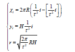
The static model of the cylindrical Fibonacci pattern of the spiral phyllotaxis is described by the system of equations [3]:

where (x_i, y_i, z_i) are the coordinates of the center of the i-th element of the pattern in 3D, R is the radius of the cylinder, H is the pitch of the blue helix genetic spiral in Figure A1.

Figure A1: Unrolling the surface of the cylinder (a) to a plane (b).

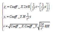
If we unroll the surface of the cylinder along the axis of symmetry to the plane, then we get a 2D phyllotactic pattern, which can be de­scribed by a system of equations:

where (x_i, y_i) are the coordinates of the center of the i-th element of the pattern, r is the radius of the elements (this formula was analytical­ly found in [3]). If you compress or stretch this pattern horizontally (Coeff_X) or vertically (Coeff_Y), you can see how the discrete elements depicted by circles “combine” into parastichies (in this case, these are straight lines), and then “fall apart”.

The program that generates frames to demonstrate this visual effect has 4 loops:

Horizontal compression (sd=0), Coeff_X decrease from 1 to 0.14;

Vertical compression (sd=1), Coeff_Y decrease from 1 to 0.14;

iii. Horizontal stretch (sd=2), Coeff_X increase from 0.14 to 1;

Vertical stretch (sd=3), Coeff_Y increase from 0.14 to 1.

The code for this program in C#:

using System;

using System.Drawing;

using System.Drawing.Imaging;

namespace Video_visual_effect

{

class Program

{

static void Main(string[] args)

{

int i, j, r, sd;//

float Coeff_X = 1, Coeff_Y = 2, Xi, Yi, PH = 100;

Color[] CCol = new Color[350];//array of element colors

PointF[] T = new PointF[330]; //array of elemet centers

int picture_X = 1920, picture_Y = 1080;// size of frame

float tau2 = (3 + (float)Math.Pow(5, 0.5)) / 2;//golden section squared

int N = 250; //250 number of elements

float Scal = 30F;//scaling factor

string name_of_out_frame;// name of out frame

Font drawFonttab = new Font(“Courier New”, 20);

SolidBrush Brtext = new SolidBrush(Color.Black);

string output_patch = “C:\\VIDEO_Visual_effect”;

System.IO.Directory.CreateDirectory(output_patch);

float R = 143F;//radius of cylinder

float H = 10.5F;//pitch of genetic the helix

for (i = 0; i < N; i++)//calculating static model array of element centers

{

T[i].X = 2F * (float)Math.PI * R * ((float)i / tau2 - (int)Math.Truncate((float)i / tau2));

T[i].Y = (float)i * H / tau2;

}

for (i = 0; i < N; i++)//coloring elements

{

CCol[i] = Color.Gray;//coloring all elements in grey;

if ((i % 3 == 2) & (i > 212) & (i < 235)) CCol[i] = Color.Orange;//coloring parastichy with index 3 in orange

if ((i % 5 == 1) & (i > 116) & (i < 190)) CCol[i] = Color.Cyan;//coloring parastichy with index 5 in cyan

if ((i % 8 == 0)) CCol[i] = Color.Blue;//coloring parastichy with index 8 in blue

if ((i % 13 == 1)) CCol[i] = Color.Red;//coloring parastichy with index 13 in red

if ((i % 21 == 0) & (i < 500) & (i > 10)) CCol[i] = Color.ForestGreen;//coloring parastichy with index 21 in green

if ((i % 34 == 19) & (i < 500) & (i > 0)) CCol[i] = Color.FromArgb(255, 255, 0, 255);//coloring parastichy with index 34 in violent

if ((i % 55 == 2) & (i < 500) & (i > 0)) CCol[i] = Color.FromArgb(255, 200, 50, 50);//coloring parastichy with index 55 in brown

}

for (sd = 0; sd < 4; sd++)// four cycles to demonstrate the visual effect

{

for (i = 0; i < N; i++)

{

if (sd == 0)// Horizontal compression, Coeff_X decrease from 1 to 0.14

{

Coeff_X = (1F - (float)i / (float)N) * .8541F + .1459F;

Coeff_Y = 1F;

}

if (sd == 1)// Vertical compression, Coeff_Y decrease from 1 to 0.14

{

Coeff_X = 0.1459F;

Coeff_Y = (1F - (float)i / (float)N) * .8541F + .1459F;

}

if (sd == 2)// Horizontal stretch, Coeff_X increase from 0.14 to 1

{

Coeff_X = (float)i / (float)N * .8541F + .1459F;

Coeff_Y = 0.1459F;

}

if (sd == 3)//Vertical stretch, Coeff_Y increase from 0.14 to 1

{

Coeff_X = 1F;

Coeff_Y = (float)i / (float)N * .8541F + .1459F;

}

PH = Coeff_X / Coeff_Y;// Stretch/Compression Ratio

Bitmap bmp = new Bitmap(picture_X, picture_Y);// open bitmap

Graphics gBmp = Graphics.FromImage(bmp);

gBmp.Clear(Color.White);

r = (int)(Math.Sqrt(Coeff_X * Coeff_Y) * Scal);// calculating radius of elements

for (j = 0; j < N; j++) // Stretch/Compression static model array of element

{

Xi = Coeff_X * T[j].X;

Yi = Coeff_Y * T[j].Y;

gBmp.FillEllipse(new SolidBrush(CCol[j]), Xi - r + 500F, Yi - r + 50F, r * 2, r * 2);// draw the circle

}

gBmp.DrawString(“Stretch/Compression Ratio”, drawFonttab, Brtext, 1450, 500);

gBmp.DrawString(PH.ToString(), drawFonttab, Brtext, 1600, 550);

name_of_out_frame = output_patch + “\\v” + (sd * N + i + 1000).ToString() + “.png”;

Console.WriteLine(name_of_out_frame.ToString());//shows program execution

bmp.Save(name_of_out_frame, ImageFormat.Png);// save frame in file

bmp.Dispose();

}

}

}

}

}

Appendix B

Explanation Video “The Biomechanical Model of Morphogenesis of Flat Spiral Phyllotaxis Patterns.”

The static model of the flat spiral Fibonacci phyllotaxis pattern is described by the system of equations [3]:

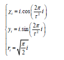
where (x_i, y_i) are the coordinates of the center of the i-th element of the pattern, ri is the radius of this element (this formula was analyt­ically found in [3]), is the base of the golden ratio, the angle of divergence of the Fibonacci phyllotaxis (also called the golden angle).

In the biomechanical model, another time variable t is added:

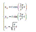
where (x_{i, t}, y_{i, t}) are the coordinates of the center of the i-th element of the pattern at time t, ri,t is the radius of this element at time t.

For the convenience of observing the growth of the phyllotaxis pattern, the author suggests coloring the element (or elements) of the pat­tern. For example, in order to highlight one parastichy with index k, it is necessary to color the elements with numbers l∙k, where l = 1, 2, 3, 4, 5….

The code for this program in C#:

using System;

using System.Drawing;

using System.Drawing.Imaging;

namespace Video_biomechanical_model

{

class Program

{

static void Main(string[] args)

{

int i, t, RX = 1920, RY = 1080;// size of frame

float x, y, dt, R, Scal;

float tau = (1F + (float)Math.Pow(5F, 0.5F)) / 2F;// golden section

float Divergence_angle = 2F * (float)Math.PI / (1F + tau);// golden angle

int N = 300; //300 number of elements

Scal = 2F;//scaling factor

string name_of_out_frame;// name of out frame

Color CC = new Color();//color of element

string output_patch = “C:\\Video_phyll”;

System.IO.Directory.CreateDirectory(output_patch);

for (t = 1; t < N; t++)//loop for adding a new element

{

for (dt = 0; dt < 1; dt = dt + 0.25F)//frames for one loop for each elements

{

Bitmap Bmp1 = new Bitmap(RX, RY); //

Graphics gBmp1 = Graphics.FromImage(Bmp1); // creat a new frame

gBmp1.Clear(Color.White); //

for (i = 1; i <= t; i++)//drawing (t-i) elements

{

CC = Color.Gray; //coloring all elements in grey;

if ((t - i) % 8 == 0) CC = Color.Red; //coloring parastichy with index 8 in red

if ((t - i) % 13 == 0) CC = Color.Green; //coloring parastichy with index 13 in green

if ((t - i) % 21 == 0) CC = Color.Cyan; //coloring parastichy with index 21 in cyan

R = Scal * (float)Math.Sqrt(Math.PI * (i + dt) / 2);// radius of element

x = Scal * (i + dt)* (float)Math.Cos(Divergence_angle * (double)(t - i));//x coordinate

y = Scal * (i + dt)* (float)Math.Sin(Divergence_angle * (double)(t - i));//y coordinate

gBmp1.FillEllipse(new SolidBrush(CC), x - R + RX / 2F, y - R + RY / 2F, R* 2F, R* 2F);// draw the circle

gBmp1.DrawEllipse(new Pen(Color.Black, 1), x - R + RX / 2F, y - R + RY / 2F, R* 2F, R * 2F);// draw border of the circle

}

name_of_out_frame = output_patch + “\\g” + (10000 + (t + dt)* 100).ToString() + “.Png”;

Console.WriteLine(name_of_out_frame);//shows program execution

Bmp1.Save(name_of_out_frame, ImageFormat.Png); // save frame in file

gBmp1.Dispose();

Bmp1.Dispose();

}

}

}

}

}