US Backscattered Detection of Layered Soft Tissues

Abstract

a) Background: US methods are applied nowadays for analyzing Soft Tissue (ST) properties. More frequently, such measurements are applied for analyzing a ST, which is behind another ST - the case analyzed in this paper. For that purpose, the Ultrasonic (US) Pressure Amplitude (PA) method was applied, followed by the analysis of the US propagation in the different media, by taking into account the relevant properties of these media, and finally find-out the US PA incident back on the Active Surface (AS) of the US transducer (that operates in a Tr/Rc mode).

b) Methods: There were analyzed here the US PA incident the AS of an US transducer, that were reflected from ST layers in the following conditions (where all the system mentioned above, was immersed in a container with Normal Saline (NS) (5%) at 25 (deg C): (1) Two homogeneous ST flat layers (μ₁, d₁) and (μ₂, d₂), with a smooth and flat interface between them; the layers were placed in series (one after the other) and the incident US was collimated. (2) The same as above, but the interface was rough, relative to the wavelength λ of the US, and (3) ST₂ was embedded in ST₁. Conditions of smooth and rough flat interface were discussed here, as well as concave or convex interface between ST₁ and ST₂: it was also discussed the condition where the incident US PA was wider than dimensions of ST₂. In most of the cases a plane interface was assumed; A concave and a convex interface were discussed as well.

c) Results: The following was concluded from the performed analytical study: (1) In case of a smooth interface, the US PA that impinges on the sensitive area of US transducer, enables to obtain the best signals with a highest SNR. (2) These condition become with lower values, due to (a) rough interface, and for (b) larger illumination than the geometrical size of ST₂; (3) This becomes even lower values for convex interface (smooth and rough); and (4) In case of a concave interface (smooth and rough) - which is dependent on its radius of curvature; (5) The optimal case of (4) is, when the radius of curvature is close (or equal) to the total distance from US transducer’s AS: at that case, most of the US PA impinges on the AS of the US transducer.

d) Conclusions: The following cases were discussed analytically in this study: (a) Homogeneous materials, different densities, smooth interface; (b) Homogeneous materials, different densities, rough interface and (c) Homogeneous materials, different densities, rough interfaces, where ST₂ is embedded in ST₁. The consistency of the obtained analytical results in this study, provide a reliable data for further analysis of other cases, which are a part of the human body.

Keywords: Soft tissue, Interface, Ultrasound, Pressure amplitude, Smooth, Rough, Convex, Concave

Introduction

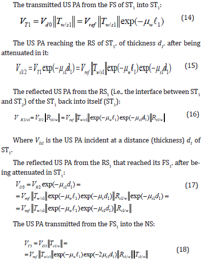
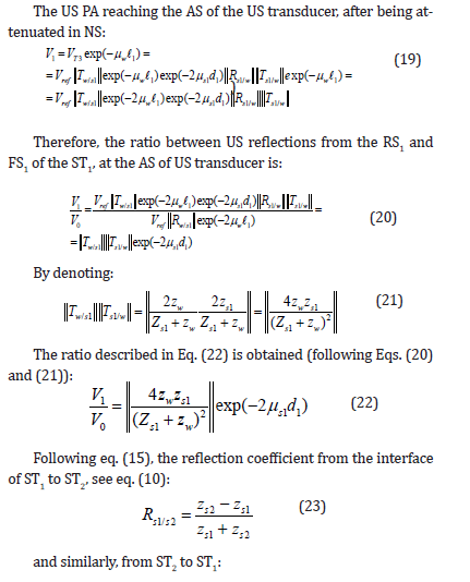
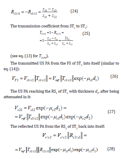
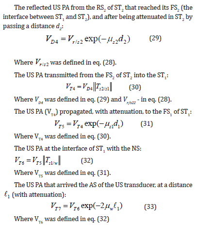
Ultrasound (US) and its monitoring methods are vasty applied for detecting Soft Tissues (STs) conditions in human body [1]. This information is followed by the analysis of the obtained data, usually 2-D images (B-scope), or 1-D images (A-scope). In these cases, the US propagates through one type of ST, until it impinges the other one, usually the ST of interest - that is to be monitored and analyzed.

Examples of detecting a ST embedded in a different STs, one can find in the following cases, which are part of a larger group/family of conditions:

I. US tests, without preliminary preparations, such as:

i. Kidneys, Urinary trach and prostate.

ii. Upper and lower part of the stomach region

iii. Genecology, including pregnancy and breasts.

iv. Eyes

v. Tongue, throat and the esophagus

II. Examples of US tests performed during a surgery:

i. Neurosurgery (like tumor in brain)

ii. Spinal cord surgery

iii. Kidneys, Urinary trach and prostate surgeries

iv. Surgeries in various parts of the upper and lower parts of the stomach region.

v. Surgeries related to various aspects of genecology and breasts.

The US methods presented here, are usually using an array of US transducers for Transmitting (Tr) US signal and Receiving (Rec) its reflected echoes. This US measurement is performed, after US propagates through a ST₁, is reflected from the interface, where starts another ST₂; Thus partially being reflected through the same ST₁ to the US transducer.

These reflections occur between the two STs, caused by the difference in their densities ρ [kg/cm³] and their US propagation velocities V [m/sec], where the product of (ρ/V) was called the im­pedance Z [(kg sec)/m²] that presents “the resistance to propagation of US wave through a tissue”; The acoustic impedance is also called as ‘the fraction of the US wave reflected from material’s surface’.

a) Techniques for ST Characterization [2]:

(i) Tensile testing. [3-6];

(ii) Compression. [7,8];

(iii) Indentation. [8-12];

(iv) Pulse wave velocity. [13-17];

(v) Pressure myography.[18-23];

(vi) Pipette aspiration. [24-27];

(vii) Elastography. [28-33];

Tables 1 and 2 in [2] summarize these measuring properties and their relative advantages.

b) ST Characterization, in case of SOS, Att., Backscatter­ing [34]. The following are the nomenclatures, characteristics and methods:

(i) UTC = US Tissue Characterization [35,36].

(ii) QUS (Quantitative US) for bone [37,38,39].

c) US Methods - to grade a normal or pathological state of an organ.

(i) Rayleigh and Love waves [40, 41] and their applications as Surface Waves [42,43].

(ii) In US Imaging systems, for distance measurements, it is assumed that the SOS = 1540 (m/sec). In reality SOS changes in the STs by ±150 m/sec, i.e., by ±10% [44, 45].

(iii) Shear waves are much slower, i.e., few m/sed in biological tissues (statistically < 10 m/sec).

(iv) For ST elasticity, Rayleigh and Love waves (< 10 m/sec) are applied.

The US testing methods, using an array of US transducers, pro­vide the information about the tested organ as a 2-D image. In this case, the quality of the image depends on the amount of the US re­ceived signal by the array of US transducers. This is because a part of the US signal propagates through ST₂, where the reflected part depends on interface quality (between the layers) and also on the incident and scattered energy from small dislocations along the path of US propagation. In this case, the “monitoring head” (that contains the US transducers and part of the ‘front-end’ electronics) is relatively large. Accordingly, when performing a measurement during a surgery, it is required a relatively large ‘opening region’ in the part of the body to be investigated - thus, the surgery has to be stopped, for making these US measurements, obtain their images and (at least) perform a preliminary interpretation; Thus, it is not a Real-Time Intra-Operative (RTIO) method.

In-order to overcome most of the limitations of the US systems described above and mainly to a surgeon, it is presented here a new US device that provides all the required data, including distance to another ST (as well as bone), by means of a RTIO method; Moreover, it is also performed with a device having small dimensions.

Methods and Results

US Backscattering in Layered Soft Tissue

The following will be discussed in this section:

(i) Homogeneous STs, different densities, smooth interface

(ii) Homogeneous STs, different densities, rough interface

(iii) Homogeneous STs, different densities, rough interfaces, where ST₂ is embedded in ST₁.

Homogeneous STs, different densities, smooth interface

In this case, there are assumed, two ST layers of thicknesses d₁ and d₂ and densities ρ₁ and ρ₂. The two ST materials are in contact with each other, and it is also assumed that the interface is smooth and planar, parallel to the FS of ST₁.

Figure 1: Describes the ‘reference’ experiment, for defining the US PA output of the US transducer (Figure 1):

Figure 1:

Figure 1: The preliminary (reference) experiment, for defining V_ref. The US transducer that operates in the Tr/Rc mode, is placed in a container, filled with Normal Saline (NS) (5%), at 25oC. Metal plate (d _{plate thickness} >10λ, where λ is the wavelength of the US waves) is placed in parallel to the Active Surface (AS) of the US transducer and at distance L1. The plate operates as a ‘total reflector’ for US waves. The NS attenuation (μw [V]) and its velocity (Vw [m·sec-1]) are measured and recorded.

Figure 2: Describes a system, for measuring the US PA on the AS of the US transducer, on which are received the reflected signals from tissues ST₁ and ST₂, when they are in contact along the inter­face (Figure 2):

Figure 2:

Figure 2: Schematic description of the measuring US PA on the AS of the US transducer from FS, RS of ST₁ and ST₂ and the inter­face between them. The US transducer operates in Tr/Rc mode, is placed in a container filled with Normal Saline (NS) (5%), at 25oC. The Front Surface (FS) of the ST₁, of thickness ‘d₁’, is parallel to the Active Surface (AS) of the US transducer and at a distance ‘ 1from it. The interface between ST₁ and ST₂ is smooth (in the 1st case), and scattering - due to its roughness (in others).

Following Figures 2:

V₀is the reflected US PA from the Front Surface (FS) of ST₁ (Fig­ure 2) [V], immediately after the reflection occurred.

V₁ is the primary reflected US PA from the Rear Surface (RS) of ST₁ (equivalent to the 1st reflection of the ST₂) (see Figure 2) [V], which is the ‘interface’ between ST₁ and ST₂.

V₂ is the reflected US PA from the RS of ST₂ (Figure 2) [V].

V₁₁ is the primary reflected US PA from the FS of the reflecting plate (Figure 1) [V]

The Attenuation (AT) coefficient of US in NS is μ_w(measured in [V]), and its SOS is V_w[m·sec^-1]. Similarly, the AT coefficient of US in STi is μ_si[V], and its SOS is V_si[m·sec^-1].

The mathematical relationship described here, is a function of the US PA, as measured by the US transducer, and is expressed in volts.

Accordingly, the distance between the front surface of the ST₁ and the US transducer (here the small dimensions of the AS of the US transducer were considered) was assumed, such that the US PA V_xpropagating in direction x is described as [46]:

V_x = V_ref· exp [-μ(f)x] (1a)

where:

V_refis US PA at the origin, at x = 0 and μi(f) is the attenuation coefficient of the media ’i’ through which the US wave propagates as a function of frequency.

μ_w is the AT coefficient of the NS [V].

R₁ is the reflection coefficient of ST₁ and R2 - of ST2.

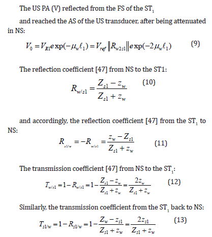
R_w/s and Rs/w are the reflection coefficients from the NS-to-ST and from ST-to-NS, respectively.

The US impedance Z is defined as the product between the US velocity V [m·sec-1] and its density ρ [kg·m-3], for a given medium.

Z_wis the US impedance of NS in the container.

Z_ST,i is the US impedance of ST No. i.

d_ST,i is the thickness of ST No. i [mm]

μ_ST,i is the AT coefficient of ST No. i [V]

T_w/STi is the transmission coefficient rom NS to STi [V]

T_ST/w is the transmission coefficient from STi to NS [V]

V_ref is the emitted US PA (V) from the US transducer.

L₁ is the distance between the AS of the US transducer to the FS of the reflecting plate [mm], (see Figure 1).

is the distance between the AS of the US transducer to the FS of the ST₁ [mm], (see Figure 2)

Assumptions:

(a) The US transducer and the ST samples (ST₁ and ST₂) are in the same container, filled with NS.

(b) The AS of the US transducer is parallel to the FS of ST₁. FS₁ of ST₁ is parallel to its RS₁; where the RS1 is the interface to FS₂ of ST₂, i.e., it is also that FS₂ and RS₂ are parallel as well.

(c) The transducer operates in the T_r/R_c mode.

(d) The US waves propagate from the AS of US transducer through the NS (with attenuation) toward the FS₁ of ST₁.

(e) The US waves are partially reflected at that interface and after propagating again through the NS (again with attenuation), they impinge the AS of the US transducer, where its PA is trans­formed to voltage V₀.

(f) The rest of the US waves are transmitted from the FS₁ and propagate through ST₁ with attenuation. On reaching the RS1 (the interface region), these US waves are partially reflected and propa­gate back; through ST₁ to its FS - where they are partially transmit­ted and propagate through the NS (with attenuation) and reach the US transducer, where they are detected and transformed to voltage V₂₁.

(g) From FS₂ of ST₂ (i.e., the interface), the US PA propagates (with attenuation) to its RS₂ and from there are reflected and reach­ing FS₂. From there, the US waves are partially reflected back and partially transmitted and propagate through ST₁ (with attenu­ation). After reaching the FS₁ (of ST₁), the US waves are partially transmitted and propagates through NS (with attenuation) toward the US transducer - thus the PA at the transducer is V₁₂.

(h) According to the described process, similar procedure oc­curs in ST₂ and its boundary regions - as it will be described in the mathematical derivation.

The Mathematical Derivation:

Presented are the mathematical derivations, for obtaining the US AT in a ST_i, by interpreting the US PA that was incident and de­tected by the US transducer. This US PA reflections arrived from the FS_s and RS_s of the Sti (here i=1, 2), and taking into consideration transmission, reflection and attenuation properties of each of the involved media. Two experiments are presented, where their out­comes are attributed by the mathematical derivations:

1. A ‘reference’ experiment.

2. The ‘soft tissues’ (STs) experiment.

The ‘Reference’ Experiment:

This experiment defines the Transmitted (Tr) US PA emitted by the AS of the US transducer, denoted by US PA V_ref.

For the described experiment, a smooth metallic plate was im­mersed in NS. The surface plate roughness < λ/20, where λ is the wavelength of the US in the NS, see Figure 1. The US wave, repre­sented by the emitted pressure V_refpropagates through the NS a dis­tance L1 (see Figure 1), taking into consideration the attenuation of the US wave in it.

The US PA (V_d0) incident the plate’s smooth surface (Figure 1) is

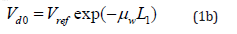
where μ_Wis the attenuation coefficient (V) of NS.

Equation (1b) is valid, under the following assumptions:

(a) The total frequency bandwidth of the US compressional wave (consisted from seven pulses) is narrow;

(b) The center frequency remains, while the high harmonics are attenuated, due to the properties of the medium they propagate through it;

(c) The detecting part of the system includes a filter, whose central frequency was matched to transmitted (Tr) frequency of the pulses.

(d) These conditions permit to perform the analysis in the way described below, by using Eq. (1a) and Eq. (1b).

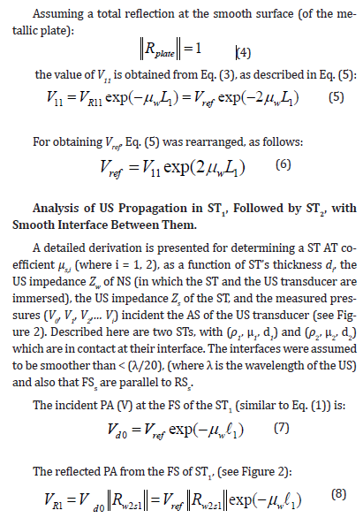
The reflected US PA from the FS of the smooth plate (immedi­ately after the US wave was reflected from it):

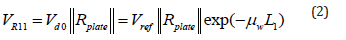
The US PA (V₁₁) at the AS of the US transducer, after it was atten­uated again in NS is described as:

Analysis of Us Propagation in ST₁ and ST₂ (Both Homoge­neous Materials), with (μ_s1, d_s1) and (μ_s2, d_s2), with a Rough In­terface Between Them

Figure 2 presents also the conditions for the analysis, where the two homogeneous materials, ST₁ and ST₂, are as in the previous case, except that their interface is rough. The roughness of the in­terface is defined as

λ/10 < roughness < λ /2

where λ is the wavelength of the applied US in these measure­ments.

Thus, the propagation phenomena and the mathematical treat­ment up to the interface, are the same as in the previous case. The US PA reaching the RS1 of ST₁, which is of thickness d₁, and after being attenuated in it, was described in eq. (15).

Types of Interface Surfaces:

(i) Assuming a random amplitude of the interface (rough­ness amplitude of λ/10, or smaller), located between ST₁ and ST₂. In this case, the reflection is Lambertian [48,49]. Thus, the reflected US PA, from the rear surface of the ST₁, while observing in a narrow cone, is close to a constant value, and with a smaller US PA, which propagates back toward the FS of ST₁.

(ii) As the interest here is in the US PA that impinges the AS of the US transducer (which is of relatively small dimensions), as­sumptions will be made according to the angular Beam-Width (BW) of the reflected lobe toward the US transducer. This US PA is always smaller than the one of a smooth interface (discussed earlier) and depends on the degree and type of a roughness.

By degree of roughness, it is meant here, the average amplitude variation of the rough surface, (relative to the US wave­length λ).

By type of roughness, it is meant (1) a random roughness (that provides a Gaussian distribution of the reflected/transmitted US PA), or (2) other types of roughness that provide several lobes in reflection (or transmission) of the US PA.

Note*: Roughness Measurements

1) Mechanical Measurement: mechanical roughness mea­surements, their statistical interpretation and some of their appli­cations, are described in [50,51];

2) Optical Interferometry: optical roughness measure­ments are described in [49,52-54]; These methods are usually ap­plied for smoother and very smooth surfaces (like diamond turning machine of polished surfaces).

3) US Methods: surface roughness measurements were also performed by applying US and developing unique methods, appli­cable in some specific applications, as described in [55-58].

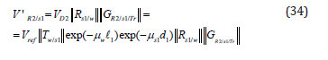
The reflected US PA from the RS1 (rough), is according and sim­ilar to Eq. (16). However, here it should be considered only the cone of US PA in the direction of the AS of the US transducer, denoted by V’R2/S1 (since reflections in other directions don’t impinge the AS of the US transducer - thus, they are not detected); therefore:

Similarly, one can calculate the US PA that reaches the AS of the US transducer, arriving from the RS of ST₂. Naturally this US PA and thus its signal, are much smaller than that from the interface of ST₁ and ST₂ (due to the ‘double attenuation’ in ST₂ along the paths d₂ and the ‘double spreading’ effects at the interface (i.e., the rough surface).

Homogeneous STs, Different Densities and Attenuations, Rough Interface, ST₂ is Embedded in ST₁:

Figure 3 presents the case, where ST₂ is located inside ST₁ and their interface is rough; where in this figure only ST₁ and ST₂ are presented and all the rest that belongs to the measuring system, is the same as in Figure 2:

Figure 3:

Figure 3: Schematic description of the geometrical interrela­tions of ST₁ and ST₂. The rest of the measuring system is the same as described in Figure 2. The US transducer operates in Tr/Rc mode, is placed in a container together with ST₁ and ST₂, which is filled with NS (5%), at 25oC. The front surface of the ST₁, of thickness ‘d₁’, is parallel to the AS of the US transducer and at a distance from it.

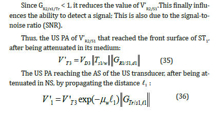
This case is similar to ‘Homogeneous materials of ST₁ and ST₂, with (μ_s1, d_s1) and (μ_s2, d_s2) and between them a rough interface’, described above as ‘case 2’; However, here the distance d’1 < d₁ as ST₂ is embedded in ST₁. Accordingly, all the equations, including eq. (34) to eq. (36), are also valid for this case, but instead of d₁ it should be changed by d’₁.

For analyzing this (third) case, the following states will be dis­cussed:

1) (a) The geometrical dimensions of ST₂ are larger than the area of US PA incident on it and (b) the impinged surface of ST₂ (by the US PA) is flat.

In this case, one obtains the same equations, including eq. (34) to eq. (36). Therefore, the US PA (detected by the US transducer) is higher, since the losses are twice reduced, due to the shorter dis­tance.Accordingly, the detected signals and the SNR are also higher.

2) The geometrical dimensions of ST₂ are larger than the US PA area incident on it and the impinged surface by the US PA is con­cave or convex.

For both types of surfaces, mentioned here, the US PA will spread (diverge) after being reflected from this kind of surfaces. The amount of the US PA that is reflected from this kind of surfaces and is incident the AS of the US transducer, depends on their curva­ture and the signal will be reduced accordingly.

However, in case of concave surfaces, that their radius of curva­ture R_curvis in the range of the focal distance R_f, i.e.

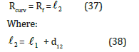
Where d₁₂is the distance between the front surface of ST₁ and the interface (i.e., the front surface of ST₂).

In these cases, the US PA incident the AS of the US transducer is increased - causing also to an improvement in the signal and the SNR.

3) The geometrical dimensions of ST₂ are smaller than the US PA area incident on it.

In this case, there exist, at least, three parts of propagation:

(a) Part of the US PA that will continue to propagate toward the rear surface of ST₁ and from there is reflected back; This case was already discussed for smooth surfaces (in #3.2). However, here is only propagating a ‘ring’ around ST₂ and accordingly are its re­flections.

(b) Part of the incident US PA impinges the rough interface, between ST₁ and ST₂, this case was also discussed above (#3.3); and

(c) Part of the incident US PA impinges the edges of ST₂, caus­

ing reflections/scattering in different and wide angular directions. Therefore, this ‘spreading effect’ of US PA, that finally part of it ar­rives to the AS of the US transducer, is a small fraction of the total reflection. Therefore, this signal is immersed in the noise, caused mainly by edge reflections and scattering.

Summarizing the above case:

The total US PA that arrives to the AS of the US transducer, is composed of three components: interface, edges and part of rear surface of ST₁. These reflections are of different types and distanc­es, thus their interpretation by the US transducer requires anapri­ori knowledge.

Summary and Conclusions

There were analyzed here the US PA incident the AS of an US transducer, that were reflected from ST layers in the following con­ditions (where all the system mentioned above, was immersed in a container with NS (5%) at 25 (deg C):

1) Two homogeneous ST of flat layers (μ1, d₁) and (μ2, d₂), with a smooth and flat interface between them; these layers were arranged in series (one after the other) and the incident US PA was collimated.

2) The same as above, but the interface was rough, relative to the wavelength λ of the US.

3) ST₂ was embedded in ST₁. Conditions of smooth and rough flat interface were discussed, as well as concave or convex interfac­es of ST₂; it was also discussed the case where the incident US PA is wider than the dimensions of ST₂.

The following was concluded from this study:

1) In case of a smooth interface, the US PA impinging on the AS of US transducer, it enabled to obtain signals with a good SNR.

2) The above-mentioned condition become worse, due to (a) rough interface, and also for (b) larger angular illumination than the geometrical dimensions of ST₂;

3) The above result becomes even worse for convex interface (smooth and rough);

4) However, in case of a concave interface (smooth and rough), the US PA on the AS of the US transducer, is dependent on the radius of curvature of the interface;

5) The optimal case in (4) is obtained, when the radius of curvature is close to the total distance from the US transducer’s AS: in that case, most of the US PA will impinge the AS of the US trans­ducer.

Acknowledgment

Sincere thanks to my late teachers and colleagues - Professors D. Zaslavsky, I. Alpan, B. Schmutter, J. Ben-Uri (all from the Technion I.I.T., Haifa, Israel), N. H. Farhat and B. D. Steinberg (both from The Moore School of E. E., U. of Pa., Phila. PA, USA), K. Biederman (IOF, KTH, Stockholm, Sweden) and R. Dandliker (Inst. of Microtechnolo­gy, Neuchatel, EPFL, Switzerland), that provided me with theability to dig into new and exciting areas of technologies and sciences.

Conflict of Interest

None.

References

• Mamou J Oelze ML (2013) Quantitative ultrasound in soft tissues. 1. Netherlands: Springer
• Kang, Kee Moon (2023) Techniques for characterizing mechanical properties of soft tissues. Journal of the Mechanical Behavior of Biomedical Materials Vol. 138: 105575.
• Mario Scholze, Sarah Safavi, Kai Chun Li, Benjamin Ondruschka, Michael Werner, et al. (2020) Standardized tensile testing of soft tissue using a 3D printed clamping system. HardwareX 21: 8: e00159
• Innocenti B, Larrieu JC, Lambert P, Pianigiani S, (2018) Automatic characterization of soft tissues material properties during mechanical tests. Muscles. Ligaments Tendons 7(4): 529-537.
• Cooney GM, Moerman KM, Takaza M, Winter DC, Simms CK (2015) Uniaxial and biaxial mechanical properties of porcine linea alba. J Mech Behav Biomed Mater 41: 68-82.
• Chow MJ, Zhang Y (2011) Changes in the mechanical and biochemical properties of aortic tissue due to cold storage. J Surg Res 171 (2): 434-442.
• Griffin M, Premakumar Y, Seifalian A, Butler P, Szarko M (2016) Biomechanical characterization of human soft tissues using indentation and tensile testing. J Vis Exp 13(118): 54872.
• Wu JZ, Cutlip RG, Andrew ME, Dong RG (2007) Simultaneous determination of the nonlinear-elastic properties of skin and subcutaneous tissue in unconfined compression tests. Skin Res Technol 13 (1): 34-42.
• Delaine Smith RM, Burney S, Balkwill FR, Knight MM (2016) Experimental validation of a flat punch indentation methodology calibrated against unconfined compression tests for determination of soft tissue biomechanics. J Mech Behav Biomed Mater 60: 401-415.
• Ansardamavandi A, Tafazzoli Shadpour M, Omidvar R, Jahanzad I (2016) Quantification of effects of cancer on elastic properties of breast tissue by Atomic Force Microscopy. J Mech Behav Biomed Mater 60: 234-242.
• Viji Babu PK, Radmacher M (2019) Mechanics of brain tissues studied by atomic force microscopy: a perspective. Front Neurosci 14:13: 600.
• Kim HL, Kim SH (2019) Pulse wave velocity in atherosclerosis. Front Cardiovasc Med 6(4): 1-13.
• Akhtar R, Sherratt MJ, Cruickshank JK, Derby B (2011) Characterizing the elastic properties of tissues. Mater Today 14 (3): 96-105.
• Vappou J, Luo J, Konofagou EE (2010) Pulse wave imaging for noninvasive and quantitative measurement of arterial stiffness in vivo. Am J Hypertens 23 (4): 393-398.
• Negoita M, Hughes AD, Parker KH, Khir AW (2018) A method for determining local pulse wave velocity in human ascending aorta from sequential ultrasound measurements of diameter and velocity. Physiol Meas 39 (11).
• Finan JD, Fox PM, Morrison B (2014) Non-ideal effects in Indentation testing of soft tissues. Biomech Model Mechanobiol 13 (3): 573-584.
• Akhtar R, Sherratt MJ, Cruickshank JK, Derby B (2011) Characterizing the elastic properties of tissues. Mater. Today 14 (3): 96-105.
• Diaz Otero JM, Garver H, Fink GD, Jackson WF, Dorrance AM (2016) Aging is associated with changes to the biomechanical properties of the posterior cerebral artery and parenchymal arterioles. Am J Physiol Heart Circ Physiol 310 (3): H365-H375.
• Markus U Wagenhäuser, Isabel N Schellinger, Takuya Yoshino, Kensuke Toyama, Yosuke Kayama, et al. (2018) Chronic nicotine exposure induces murine aortic remodeling and stiffness segmentation-implications for abdominal aortic aneurysm susceptibility. Front Physiol 31:9: 1459.
• Ogalla E, Claro C, Alvarez de Sotomayor M, Herrera MD, Rodriguez Rodriguez, R (2015) Structural, mechanical and myogenic properties of small mesenteric arteries from ApoE KO mice: characterization and effects of virgin olive oil diets. Atherosclerosis 238 (1): 55-63.
• Myrthe M Van Der Bruggen, Koen D Reesink, Paul J M Spronck, Nicole Bitsch, Jeroen Hameleers, et al (2021) An integrated set-up for ex vivo characterization of biaxial murine artery biomechanics under pulsatile conditions. Sci Rep 11 (1): 2671.
• Lawton PF, Lee MD, Saunter CD, Girkin JM, McCarron JG, Wilson C (2019) VasoTracker, a low-cost and open-source pressure myograph system for vascular physiology. Front Physiol 10: 1-17.
• Buffinton CM, Tong KJ, Blaho RA, Buffinton EM, Ebenstein DM (2015) Comparison of mechanical testing methods for biomaterials: pipette aspiration, nanoindentation, and macroscale testing. J Mech Behav Biomed Mater 51: 367-379.
• Ozawa H, Matsumoto T, Ohashi T, Sato M, Kokubun S (2001) Comparison of spinal cord gray matter and white matter softness: measurement by pipette aspiration method. J Neurosurg 95: 221-224.
• Ohashi T, Abe H, Matsumoto T, Sato M (2005) Pipette aspiration technique for the measurement of nonlinear and anisotropic mechanical properties of blood vessel walls under biaxial stretch. J Biomech 38(11): 2248-2256.
• Scheible F, Lamprecht R, Semmler M, Sutor A (2021) Dynamic biomechanical analysis of vocal folds using pipette aspiration technique. Sensors 21(9): 1-19.
• Liu F, Tschumperlin DJ (2011) Micro-mechanical characterization of lung tissue using atomic force microscopy. J Vis Exp 28(54): 2911.
• Gennisson JL, Deffieux T, Fink M, Tanter M (2013) Ultrasound elastography: principles and techniques. Elsevier Masson SAS Diagnos. Intervent Imag 94 (5): 487-495.
• Sigrist RMS, Liau J, El Kaffas A, Chammas MC, Willmann JK (2017) Ultrasound elastography: review of techniques and clinical applications. Theranostics 7(5): 1303-1329.
• Tomasz J Czernuszewicz, Jonathon W Homeister, Melissa C Caughey, Mark A Farber, Joseph J Fulton, et al. (2015) Non-invasive in-vivo characterization of human carotid plaques with acoustic radiation force impulse ultrasound: comparison with histology after endarterectomy. Ultrasound Med Biol 41(3): 685-697.
• Herman J, Sedlackova Z, Vachutka J, Furst T, Salzman R, et al. (2017) Shear wave elastography parameters of normal soft tissues of the neck. Biomed Pap 161(3): 320-325.
• Clarke EC, Cheng S, Green M, Sinkus R, Bilston LE, et al. (2011) Using static preload with magnetic resonance elastography to estimate large strain viscoelastic properties of bovine liver. J Biomech 44(13): 2461-2465.
• Linzer M (1976) The ultrasonic tissue characterization seminar: an assessment. J Clin Ultrasound 4(2): 97-100.
• Guy Cloutier, Francois Destrempes, Francois Yu, An Tang (2021) Quantitative ultrasound imaging of soft biological tissues: a primer for radiologists and medical physicists. Cloutier et al. Insights Imaging 12(1): 127.
• Zhou Z, Wu W, Wu S, Jia K, Tsui PH, et al. (2017) A review of ultrasound tissue characterization with mean Scatterer spacing. Ultrason Imaging 39(5): 263-282.
• Docking SI, Cook J (2016) Pathological tendons maintain sufficient aligned fibrillar structure on ultrasound tissue characterization (UTC). Scand J Med Sci Sports 26(6): 675-683.
• Gluer CC (1997) Quantitative ultrasound techniques for the assessment of osteoporosis: expert agreement on current status. The International Quantitative Ultrasound Consensus Group. J Bone Miner Res 12(8): 1280-1288.
• Njeh CF, Boivin CM, Langton CM (1997) The role of ultrasound in the assessment of osteoporosis: a review. Osteoporos Int 7(1): 7-22.
• Landau LD, Lifshitz EM (2002) Theory of elasticity. 3 Oxford: Butterworth Heinemann.
• Morse PM, Ingard KU (1986) Theoretical acoustics. New Jersey: Princeton University Press.
• Nenadic IZ, Urban MW, Aristizabal S, Mitchell SA, Humphrey TC, et al. (2011) On Lamb and Rayleigh wave convergence in viscoelastic tissues. Phys Med Biol. 56(20): 6723-6738.
• Shih CC, Qian X, Ma T, Zhaolong Han, Chih-Chung Huang, et al. (1898) Quantitative assessment of thin-layer tissue viscoelastic properties using ultrasonic micro-elastography with lamb wave model. IEEE Trans Med Imaging 37(8): 1887-1898.
• Goss SA, Johnston RL, Dunn F (1980) Compilation of empirical ultrasonic properties of mammalian tissues II. J Acoust Soc Am 68(1): 93-108.
• Anderson ME, McKeag MS, Trahey GE (2000) The impact of sound speed errors on medical ultrasound imaging. J Acoust Soc Am 107(6): 3540-3548.
• Christian M Langton, Christopher F Njeh (2008) The measurement of Broadband Ultrasonic Attenuation in cancellous bone - A review of the science and technology. IEEE Trans of Ultrasonics Ferroelectronics and Frequency Control 55(7): 1546-1554.
• Lawrence E Kinsler, Austin R Frey, Allen B, Coppers, James V Sanders, et al. (1999) Fundamental of Acoustics, 4th Edition. John Wiley Sons Inc.
• Angel Edward (2003) Interactive Computer Graphics: A Top-Down Approach Using OpenGL (third ed.).
• Keelan Robert, Shimada Kenji, Rabin Yoed (2016) GPU-Based Simulation of Ultrasound Imaging Artifacts for Cryosurgery Training. Technology in Cancer Research Treatment 16(1): 5-14.
• D Pantzer, J Politch, L Ek (1986) Heterodyne profiling instrument for the angstrom region. Applied optics 25(22): 4168-4172.
• Nowicki B (1986) Surface roughness and measurement with new contact methods. Intl J Mech Tool Design Res 26(1): 61-68.
• misumi-ec.com/prof/tech/press/pr1167-1168.pdf
• J Politch, D Pantzer (1988) Influence of a converging incident beam and variations in the surface complex index of refraction on optical profilometric measurements. Applied optics 27(15): 3185-3189.
• J Politch (1989) Profilometry in The Angstrom Region. Optical Testing and Metrology II 954: 292-299.
• J Politch (1989) Optical Measurements of Diamond-Turned Surfaces. 6^th Mtg in Israel on Optical Engineering 1038: 260.
• (2005) Application of Air-Coupled Ultrasound to Noncontact Surface Roughness Evaluation. Japanese Journal of Applied Physics 44(6B): 4417-4420.
• RS Dwyer Joyce, BW Drinkwater, AM Quinn (2001) The Use of Ultrasound in the Investigation of Rough Surface Interfaces. Transactions of the ASME 123(1).
• Gerald V Blessing, John A Slotwinski, Donald G Eitzen, Harry M Ryan (1993) Ultrasonic measurements of surface roughness. Appl Opt 32(19).
• Nagy PB, Rose JH (1993) Surface roughness and the US detection of subsurface scatterers. J Appl Phys 73(2): 566-580.