Modified Inelastic Buckling Load Equations for Tapered Members

Abstract

Inelastic column buckling as opposed to elastic column buckling occurs when the compressive stress locally exceeds the yield strength over a portion of the cross-section typically due to residual stresses, out-of-plane straightness, and accidental moments causing a reduction in member stiffness. Fiber based models and finite element models are used to study the variation of stress in the cross-section when subjected to axial compressive load and to predict the elastic and inelastic buckling capacity. For the fiber-based models, two types of models were developed. One model is for a prismatic member consisting of a built-up section with four angles and batten plates. This model is used to predict the inelastic buckling load using fiber analysis compared directly to the equations in the AISC “Specifications for Structural Steel Buildings” (2010) Chapter E. The equations in AISC are for prismatic members and therefore this model validates the analytical procedure. The second model is for the tapered built-up cross-section. The results are compared to a modified version of the equations presented in AISC (2010) (modified from the equations in AISC, Chapter E) for tapered members.

Finally, the finite element models were expanded to analyze inelastic column buckling. The models that were used to determine the elastic buckling loads with an eigenvalue analysis were used to establish an initial buckled shape. Then, compressive load was applied to columns that had initial residual stresses. The finite element models further validated the fiber models for tapered columns which was necessary due to uncertainties in the methodology.

Keywords: Tapered Member, Inelastic Buckling, Elastic Critical load, Residual Stress, Fiber Analysis, Finite Element Analysis, Modified AISC Equations

Introduction

Several theories have been developed for inelastic buckling; the tangent-modulus theory, the reduced-modulus theory, and Shanley’s theory (Shanley 1947) [8]. Shanley performed experimental investigations and compared the results to a mathematical analysis and found that inelastic buckling did not have a unique critical load. Also, Shanley indicates that the two extremes of the inelastic buckling are the tangent-modulus theory and the reduced-modulus theory.

According to the theory, the tangent-modulus and reduced-modulus critical loads are only the upper and lower boundaries of an infinite number of possible buckling loads. This theory indicates that inelastic buckling is determined by the relative rates of vertical loading and bending in the buckling process. When a column starts to deflect laterally, the stresses and strains through its cross-section due to both vertical compression and bending is superimposed. If the axial strain is more prudent than the flexural strain, it is possible for buckling to occur without strain reversal. If the column deflects rapidly such that only strain reversal on its convex face keeps the load constant, then the process described as the reduced-modulus theory occurs.

Yura (Yura 1971) [9] derived a stiffness reduction factor for prismatic columns when differentiating between elastic and inelastic buckling. The author assumed that the stiffness of the column in the inelastic range can be taken as proportional to a reduced stiffness, E_TI, where E_T is the tangent modulus. Yura indicated that the ratio of the inelastic critical buckling stress, F_cr,inelastic, to the elastic critical buckling stress, F_cr,inelastic, is equivalent to the ratio of the tangent modulus to the elastic modulus. These relationships were used to determine a stiffness reduction factor. Due to the elastic and inelastic behavior, an adjustment in the design criterion of the prismatic column was applied using this study. When the slenderness ratio indicates that the column should fail by inelastic column buckling, the relative stiffness ratio, G_elastic, is multiplied by the stiffness reduction factor,ET/E,

In a historical review, Bjorhovde (Bjorhovde 1988) [5] mentioned that in 1889, Considered and Engesser concluded that Euler’s formula was valid only for slender columns and inelastic column buckling should be considered for short columns. Also, the author mentioned that Considered and Engesser suggested that in order to apply Euler’s formula to short columns, the constant tangent modulus E should be replaced by an effective modulus, E_t= 0.8τ_bE, that depends upon the magnitude of stress at buckling. Bjorhovde indicated that Engesser extended the elastic column buckling theory in 1889 assuming that inelastic buckling occurs with no increase in load, and the relation between stress and strain is defined by tangent modulus E_T. Bjorhovde discussed the development of practical column design formulae and approaches based on test results and statistical analyses. The author compared the tangent modulus load and the reduced modulus load graphically based on test results data for several columns with out-of-straightness as shown in Figure 1. The tangent modulus load was shown to be a 3 lower bound, and the reduced modulus load was an upper bound only attainable under ideal circumstances.

Figure 1: Bands of maximum column strength curves (Bjorhovde 1988).

Fiber Based Model and Residual Stresses

In the fiber analysis model, when some of the cross-section yields, an effective moment of inertia is calculated corresponding to the moment of inertia of the rest of the cross section in which the material still has stiffness. This effective moment of inertia is used to predict the buckling capacity.

When a steel column is subjected to a compressive load, there are a number of limits states that may cause failure; inelastic column buckling, elastic buckling, and local buckling of plate elements. The governing failure mechanism as well as the critical buckling load depends on the unbraced length, boundary conditions, slenderness of individual plate elements, strength, and stiffness.

The cross-section that was idealized to develop a fiber-based model is shown in Figure 2 and is a built-up shape consisting of four angles assumed connected by batten plates. Each angle leg is 3 in. and has a thickness of 0.5 in. Figure 3 also shows the initial residual stress pattern that was assumed in the cross-section due to fabrication. On each leg, the maximum compressive residual stress at the tip is assumed to be 12 ksi and the maximum tensile residual stress where the legs meet is 12 ksi. Residual stresses are often due to uneven cooling during the fabrication process. It is common that compressive residual stresses develop at the tips of flanges and tensile residual stresses develop at the k-region (where legs meet). It is critical to assume that the summation of forces in the cross-section is equal to zero for equilibrium prior to applied load. The yield strength of 36 ksi was used to determine the maximum value of the compressive and tensile residual stress which is assumed 33% of the yield stress. In Section F2 of the commentary of AISC (AISC 2012), it is noted that the assumed residual stress is taken as 0.3F_y (30%) for flexural members and when differentiating between inelastic lateral torsional buckling and elastic lateral torsional buckling. Therefore, a similar assumption is used in this analysis.

For the fiber-based model, the cross-section is discretized into a number of fibers. Each fiber has an area and a distance from the neutral axis which is used to calculate the moment of inertia of the cross-section and later used to calculate an effective moment of inertia of the cross-section. The model which consists of four angles is divided into 1600 fibers. Each angle has 400 fibers and therefore, each leg has 200 fibers. Based on the residual stress pattern, each fiber is designated with its own initial residual stress assumed constant within the fiber.

Figure 2: Fiber discretization over the cross-section and residual stresses.

Analytical Procedure for Fiber-Based Model of Prismatic Member

The fiber analysis method is used to analyze the built-up section for compressive capacity considering inelastic and elastic failure modes. The yield stress of the built-up section is assumed 36 ksi. The maximum residual stress is assumed 12 ksi, compression or tension. Therefore, when a compressive load is applied that corresponds to a uniform compressive stress of 24 ksi, the angle’s leg tips begin to yield. An elastic-perfectly plastic stress strain curve is assumed in each fiber as shown in Figure 3. When the fibers yield, they no longer contribute to the flexural stiffness of the cross-section as evident from Figure 3. Therefore, a new effective moment of inertia needs to be calculated for the cross-section.

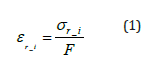
One primary assumption in the fiber analysis is that the cross-section deforms uniformly after load is applied. Therefore, the fiber analysis was strain controlled and the strain in the cross-section due to applied load was assumed constant. The initial residual strain was computed for each fiber i using Equation 1 where ε_{r_i} is the initial residual strain in each fiber, σ_{r_i} is the initial residual stress interpreted from Figure 3, and E is the elastic modulus equal to 29000 ksi.

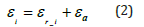
Load was applied in the fiber model by adding a uniform axial compressive strain in the cross-section. This strain is denoted as ε_a and it is assumed that compression is positive in the analysis. Therefore, the new strain for each fiber  after load is applied, ε_i is computed using Equation 2.

If ε_i is computed greater than or equal to the yield strain, ε_y, then the fiber has yielded, and the stress in the fiber, σ_i, is equal to the yield stress. The yield strain is computed in Equation 3. If the strain is less than the yield strain, then the fiber is behaving elastically, and the stress is computed using Equation 4.

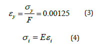
The total applied load on the cross section is equal to the summation of the values that are obtained by multiplying the stress on each fiber by the fiber area (0.0075 in2 from Figure 2). This is illustrated using Equation 5 where A_i is the area of each fiber and P_i is the load within each fiber. load within each fiber.

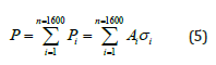
Figure 3: Stress-Strain relation before and after yielding.

Assuming the column fails by inelastic column buckling; as more load is applied, the effective stiffness decreases, thus decreasing the buckling capacity. The correct buckling load is obtained when the applied load which causes part of the cross-section to yield is equal to the critical buckling load, P_cr which considers the reduced stiffness.

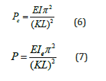
For a prismatic member, the elastic buckling capacity is obtained using Equation 6. In the fiber-based model, the moment of inertia, I, is obtained from the summation of the moment of inertia contribution for each fiber which considers the distance from the neutral axis of the cross section. When a portion of the cross-section yields due to residual stresses prior to buckling, an effective moment of inertia, I_e is calculated by assuming the moment of inertia contribution of the yielded fibers is zero. The critical buckling load is computed using Equation 7 which can also be used if the entire cross-section remains elastic.

Values of the critical buckling load, P_cr are plotted for different slenderness ratios, KL/r, and compared to the critical buckling loads obtained using AISC equations (AISC 2010).

Prismatic Member Results and Comparisons to AISC

Equation 7 was used to plot the critical loads for different effective lengths. The results are presented in Figure 3 (Fiber Analysis Results) which is discussed further in the proceeding paragraphs.

Figure 4: Comparison between Fiber Analysis and AISC Results for prismatic member.

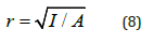
In Figure 4, the critical load is plotted vs. the slenderness ratio defined as KL/r, where r is the radius of gyration corresponding to the entire cross-section and is calculated using Equation 8. Therefore, after the critical buckling loads were determined for different effective lengths, the effective lengths were divided by the radius of gyration for graphing purposes and to compare to AISC equations.

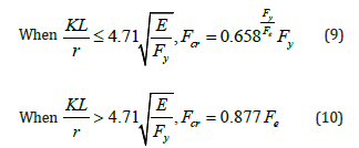
AISC (2012) provides two equations for calculating the critical buckling stress, F_cr, for doubly symmetric prismatic members with non-compact plate elements only. These equations are within Section E3 of the specification. The equation that is used is dependent on the slenderness ratio and whether it is assumed the column buckles elastically or inelastically. Equation 9 is used for inelastic buckling and Equation 10 is used for elastic buckling.

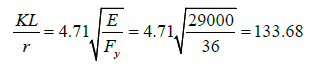
The slenderness ratio limit, KL/r, which determines whether this cross-section fails by elastic or inelastic buckling for a yield stress of 36 ksi is calculated as follows:

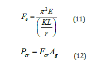
The elastic buckling stress, F_e, from Equations 9 and Equation 10 is computed using Equation 11 and the critical buckling load is computed using Equation 12.

In Equation 10, the 0.877 factor accounts for imperfections in the geometry which were not considered in the fiber analysis model. However, the influence of imperfections, out-of-plane straightness and eccentricities does not show up directly in Equation 9. It is assumed that considerations for imperfections in a tapered column should be the same as that in a prismatic column. Therefore, for comparison purposes,

the fiber analysis results are multiplied by 0.877 and compared in Figure 4 as well (Fiber Analysis x 0.877). However, the results do not compare well when the slenderness ratio is low.

AISC Inelastic Column Buckling Discussion

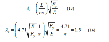
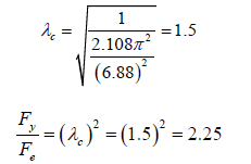
In AISC (2012), a best fit curve was used to develop a relationship between a slenderness parameter and the ratio of critical stress to yield stress. This best fit curve is graphed based on experimental data as shown in Figure 5 (Hall 1981) [7]. The limit that separates elastic and inelastic buckling is represented by the slenderness ratio, , and by a slenderness parameterc λ_c equal to 1.5. The slenderness parameter is calculated using Equation 13 and the value of 1.5 is calculated using Equation 14.

Figure 5: Relation between λ_c and / F_cr/F_y using experimental data (Hall 1981).

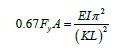
Although the limit of was fitted using experimental data, a similar value can be derived assuming the residual stress pattern in Figure 2. The residual stresses are 33% of the yield stress. Therefore, when the applied stress is more than 67% of the yield stress or when the applied load corresponds to more than 67% of F_yA, the column will fail by inelastic buckling in lieu of elastic buckling. Using Equation 6, the limit is derived as follows:

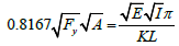
Taking the square root of both sides:

Moving terms:

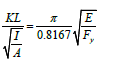
Finally, by using Equation 8, Equation 15 is obtained:

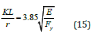
The value of 3.85 is lower than the value of 4.71. Other issues involving inelastic buckling that influence this value include out-of-plane straightness and eccentricities which introduce secondary moments. The value of 4.71 corresponds to a stress of 0.44F_y in lieu of 0.67F_y. However, this procedure and relationship discrepancies between the values can be used to formulate a recommended design curve that corresponds to inelastic buckling of tapered columns.

Fiber Analysis of Tapered Member

The fiber analysis for a prismatic member is repeated for the tapered built-up member with a tapering ratio, u = 2, and a shape factor, m = 2, that is shown in Figure 6.

Figure 6: Non-prismatic beam-column element (Al-Sarraf 1979).

Where:

a_o = the distance from the origin O to the smaller member depth

b_o = the distance from the origin O to the larger member depth

d₁ = the depth at larger member depth between the centroid of angles

d₂ = the depth at smaller member depth between the centroid of angles

u = tapering ratio b_o/a_o or d1/d2 (Figure 6)

A₁ = the cross-section area at larger member depth (4A_angle)

A₂ = the cross-section area at smaller member depth (4_Aangle)

A_angle = cross sectional area of one angle

I₁ = the moment of inertia at larger member depth [4(I_angle + A_angle d₁ ² /4)]

I₂ = the moment of inertia at smaller member depth [4(I_angle + A_angle d₂ ² /4)]

I_angle = moment of inertia of one angle

O = the vanishing point of the tapered member

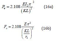
The flexural buckling limit state for a tapered member is not available in AISC (2012) or any other references. Therefore, a new set of equations for elastic and inelastic buckling is derived using the fiber analysis and other information developed in (Bukaita 2013) [6]. Equation 16a represents the elastic buckling load while Equation 16b represents the elastic buckling stress for a tapered column with a tapering ratio, u=2, and a shape factor, m=2.

Assuming the residual stress pattern in Figure 2, the following applied load is that required to initiate yielding of the cross-section.

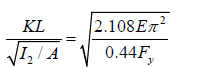
The actual limit that differentiates between elastic and inelastic buckling for a prismatic member assumes that the applied stress is 0.44F_y. Therefore, the recommendations for tapered columns will be the same. The assumed load that would initiate yielding is modified using Equation 17.

By equating Equation 16 with Equation 17:

Dividing both sides by 0.44 and moving terms:

Taking the square root of both sides:

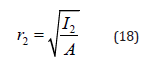
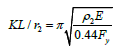
The value of r2 represents the radius of gyration at the smaller member depth and is calculated using Equation 18.

Finally, Equation 19 is obtained.

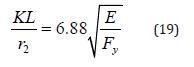
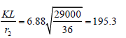
The expression to the right is assumed to be the slenderness limit that separates between elastic and inelastic buckling of the tapered member. Assuming that the yield stress of the member is 36 ksi, the limit is:

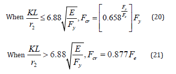
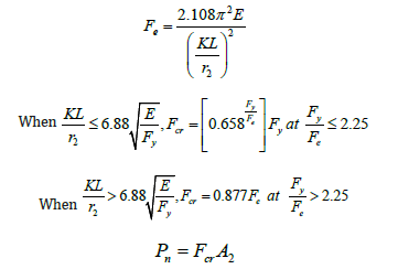
Equations 20 and 21 represent the modified AISC equations for the tapered member in question. In general, the modified equations are very similar to Equations E3-2 and E3-3 in AISC (2010). The primary differences are; [1] the limit that determines which equations to use, [2] the calculation of F_e, and [3] using the radius of gyration at the smaller member end only, r₂.

The slenderness parameter is defined using Equation 22.

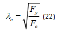
By substituting Equation 16b into Equation 22, Equation 23 is obtained.

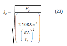
By substituting Equation 19 into Equation 23, Equation 24 is obtained.

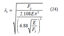
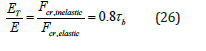
Simplifying Equation 24, the slenderness parameter that separates elastic and inelastic buckling is obtained. Also, the ratio Fy/Fe is obtained.

The elastic buckling stress, Fe, from Equations 20 and Equation 21 is computed using Equation 16b. The critical buckling load is computed using Equation 25.

The results of the fiber analysis are compared to the results of the modified AISC equations (Equations 20 to 25) in Figure 6. As in Figure 4, the fiber analysis results are multiplied by 0.877 for further comparisons to the modified AISC equations. The results indicate that the modified equations underestimate the critical buckling load in comparison to the fiber analysis. However, the fiber analysis results multiplied by 0.877 compare well for slenderness ratios of 75 and higher. This was also evident from the results provided in Figure 4 for a prismatic member. Overall, the comparisons in Figure 4 for a prismatic member are very similar to the comparisons in Figure 7 for the tapered member. Therefore, the new modified equations for tapered members compare favorably to the equations currently presented in AISC for a prismatic member and the only modifications recommended are [1] the computation of F_e and [2] the slenderness ratio that differentiates between elastic and inelastic column buckling.

Figure 7: Results of Fiber Analysis and modified AISC equations for tapered Member.

ABAQUS Analysis of Tapered Member

The finite element approach is the second analysis method used to obtain the elastic and inelastic buckling loads for the tapered member in question. This approach was used to validate the methodology of the fiber models due to uncertainties in the load carried by the inelastic column at buckling.

The built-up tapered model dimensions and shape described above is used for the finite element model. The model consists of 5252 nodes and 4900 shell elements to represent the 4 angles. Another 100 square elements were used to represent the batten. The tapered built-up column includes four [4] 3 in. x 3 in. x ½ in. angles that were connected by the batten plates along the length. The cross-sectional dimensions are 10 x 10 in. centroid-to-centroid of the steel angles at the smaller member depth and 20 in. x 20 in. at the larger member depth. Therefore, the tapering ratio of all selected models is equal to 2.

Eight different member lengths (300 inches to 4000 inches) for fixed-fixed support conditions and another five different member lengths (300 inches to 2000 inches) for hinged-hinged support conditions were analyzed and compared with fiber analysis results. The distance between battens is designed to be constant and equal to 0.01L as shown in Figure 8. A short distance between the battens eliminates the shear effect.

Figure 8: The built-up tapered batten model under consideration.

Development of Finite Elements Models

The analysis was performed as a static-stress analysis using the *Static Riks option which can be used to study the post-buckling behavior. In this type of analysis, the finite element model does not buckle naturally if the column is perfectly straight. Instead, it is necessary to insert an imperfection into the model. An imperfection of 10% of the buckled shapes from the eigenvalue analysis was used.

Since inelastic deformations are expected, it is necessary to specify that when the yield strain is exceeded, the stress is equal to the yield stress (normal stress example). This was incorporated in the ABAQUS model using the *Plastic option. The initial residual stress pattern was implemented into the finite element model using the *Initial Conditions Type = Stress option. Fewer elements within the cross-section were used in the finite element model in comparison to the fiber model.

The analysis results from the finite element models are divided into two groups depending on boundary conditions. For each model, two input files are created. One is used to obtain the eigenvalue results and the other is used to obtain the buckling load considering the initial residual stresses. The eigenvalue results are stored in a temporary file for the “Imperfection” inserted into the second file.

Fixed-Fixed Boundary Conditions

The first model is the built-up tapered member with a 300 in. length. Figure 9 shows the applied load vs. time history. From this figure, it is determined that the maximum load of 425.8 kips is obtained prior to the column buckling inelastically.

The second model is the built-up tapered member with an 800 in. length. Figure 10 shows the applied load vs. time history. From this figure, it is determined that the maximum load of 410.2 kips is obtained prior to the column buckling inelastically.

Figure 9: Applied load vs. Arc Length, length=300 in., fixed-fixed.

Figure 10: Applied load vs. Arc Length, length=800 in., fixed-fixed.

ABAQUS Results

Similar charts were made for lengths of 1200 in., 1600 in., 2000 in., 2400 in., 3000 in., and 4000 in. The maximum loads were determined to be 369 kips, 274 kips, 180 kips, 126 kips, 81 kips, and 46 kips, respectively.

Figure 11: Applied load vs. Arc Length, length=300 in., hinged-hinged.

Hinged-Hinged Boundary Conditions

The first model is the built-up tapered member with a 300 in. length. Figure 11 shows the applied load vs. time history. From this figure, it is determined that the maximum load of 411 kips is obtained prior to the column buckling inelastically.

The second model is the built-up tapered member with a 600 in. length. Figure 12 shows the applied load vs. time history. From this figure, it is determined that the maximum load of 350 kips is obtained prior to the column buckling inelastically.

Figure 12: Applied load vs. Arc Length, length=300 in., hinged-hinged.

Similar charts were made for lengths of 1200 in., 1600 in., and 2000 in. The maximum loads were determined to be 126 kips, 75 kips, and 42 kips, respectively. Figure 13 shows the complete load-displacement relationships for all lengths and with fixed-fixed boundary conditions. Figure 14 shows the complete load-displacement relationships for all lengths and with hinged-hinged boundary conditions. The values for each curve represent the lengths of each model.

Analysis Results and Comparisons

Figure 15 compares the finite elements results to the fiber analysis results for a tapered column with fixed-fixed support conditions. The slenderness ratio is used in lieu of the length. Figure 16 compares the finite elements results to the fiber analysis results for a tapered column with hinged-hinged support conditions. Overall, the comparisons are favorable and even better than anticipated considering the reduction in elements in the finite element model. This study validates the work performed in this study and recommendations that are provided for the design capacity of tapered columns as well as the alignment charts.

Figure 13: Load-Displacement by using ABAQUS for 8 lengths with fixed-fixed support conditions.

Figure 14: Load-Displacement by using ABAQUS for 5 lengths with hingedhinged support conditions.

Figure 15: Comparison between Fiber Analysis Results and ABAQUS Results, for fixed-fixed support condition.

Figure 16: Comparison between Fiber Analysis Results and ABAQUS Results, for hinged-hinged support condition.

Stiffness Reduction Factor

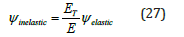
The alignment charts that are derived for built-up tapered member (Bukaita 2013) that are shown in appendix A cannot be used for inelastic buckling without considering the reduced stiffness when calculating the relative stiffness ratio at larger and smaller member depth ψ₁ and ψ₂. These alignment charts as well as the AISC alignment charts are derived based on elastic behavior. A stiffness reduction factor should be multiplied by the relative stiffness ratio to obtain a new relative stiffness ratio for tapered members when Equation 9 is used in lieu of Equation 10. It is proposed that the same reduction factor used to reduce the stiffness of a prismatic column is used to reduce the stiffness of the tapered column. The stiffness reduction factor is obtained using Equation 26.

The relative stiffness ratio for the tapered member under inelastic effect can be obtained using Equation 27 modified which is the same of the modified relative stiffness ratio for a prismatic member when subjected to inelastic buckling.

Conclusions

Due to the variation of residual stresses in the cross-section, part of the cross-section may yield prior to buckling. Therefore, the buckling load capacity is reduced due to a reduction in the effective moment of inertia. Some observations and conclusions considering the influence of residual stresses and other imperfections in tapered columns are summarized as follows:

a) For a prismatic member and according to AISC (2010), the slenderness ratio that separates between inelastic buckling and elastic buckling is which assumes the maximum stress before yielding due to applied load only is 0.44F_y.

b) For the tapered member with tapering ratio u = 2, the slenderness ratio that separates between inelastic buckling and elastic buckling is equal to 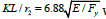which assumes that the maximum stress before yielding is 0.44F_y.

c) In general, for other tapering ratio, the slenderness ratio that separates between inelastic buckling and elastic buckling assuming the same stress before yielding can be obtained with respect to the non-dimensional axial force parameter for the particular tapered column:

d) The slenderness parameterfor the tapered member is equal to the slenderness parameter for a prismatic member (1.5).

To determine the compressive capacity of tapered columns, the following modified equations are recommended for a tapering ratio u = 2 and with a built-up cross-section. More modified equations are required for other cross-sections and other tapering ratios.

Finite element models were used to verify the results using an eigenvalue approach and several boundary conditions. This procedure can be idealized for other tapered columns and alterations are required for each type of tapered column and each tapering ratio.

In the fiber analysis models and finite element models, the initial residual stress pattern in the cross-section was similar to residual stress patterns assumed by AISC (2010).

Compressive residual stresses were assumed at the leg tips of the angles and tensile residual stresses were assumed near the k-region (i.e. where the angle legs meet). The residual stresses are assumed constant throughout the entire length.

The critical buckling stress for a prismatic member is computed in AISC (2010) using Section E3 and Equations E3-2 and E3-3. Equation E3-2 is for when inelastic buckling is expected and Equation E3-3 is for when elastic buckling is expected. In order to evaluate the practicality of the new alignment chart and derivation of the buckling load for a tapered column, the derivation had to be evaluated when subjected to inelastic stresses.

APPENDIX A

Figure A-1: Alignment chart for braced frame against side sway at u=2.

Figure A-2: Alignment chart for braced frame against side sway at u=4.

Figure A-3: Alignment for unbraced frame against side sway at u=2.

Figure A-4: Alignment for unbraced frame against side sway at u=4.

References

• ABAQUS (2011) ABAQUS 6.11/CAE User’s Manual/Standard User’s Manuals Modeling and Visualization Analysis: Volumes I-V, Online documentation HTML format.
• AISC (2010) Specification for Structural Steel Buildings, American Institute of Steel Construction, Chicago, IL.
• AISC (2012). Manual of Steel Construction, fourteenth Edition. American Institute of Steel Construction, Chicago, IL.
• Al Sarraf SZ (1979) Elastic Instability of Frames with Uniformly Tapered Members, The Structural Engineer, March pp 18.
• Bjorhovde, Reidar (1988) American Institute of Steel Construction, First Quarter, pp 21-30. Columns from Theory to Practice, Engineering Journal.
• Bukaita, Wisam V (2013) Development of Analytical Design Procedures for Tapered Columns, Thesis, Lawrence Technology USA.
• Hall DH (1981) Proposed Steel Column Strength Criteria, Journal of Structure, merican Institute of Steel Construction, Vol. 107, No. ST4 pp 649-670.
• Shanley FR (1947) Inelastic column theory, Journal of the Aeronautical Sciences pp. 261-268.
• Yuar JA (1971) The Effective Length of Columns in Unbraced Frames, Engineering Journal, Vol (8) No 2, Second Quarter, pp. 37 - 42.