An Overview of the Perspective MLM-Applications to Theoretical Aspects of the Radiation Therapies

Abstract

In [1] (i.e., the year 2024 “Proton Therapy – Scientific Questions and Future Direction” edited by TJ FitzGerald), the Multi-Level Model (= MLM) was outlined as a conceptual framework proposed by Levichev. In particular, we presented there, in our perspective chapter ([2]), the proton’s theoretical description in an endeavor of its future application in proton therapy for cancer patients. This exploration potentially opens a novel era of the intricate interplay between wave functions (mathematically, they form an infinite-dimensional space Fp, see [3]) and proton beams produced by different vaults. An overview of this chapter, as well as of certain recent findings of Fp–elements, is part of the talk. Besides, due to the mere scope of the MLM-approach, it is now expected to be applied in a broader context (rather than within proton therapy, alone). The MLM becomes, so to say, part of the holistic medicine approach.

An Overview of [2], “The Proton’s Theoretical Description Based on Wigner-Segal Approach to Elementary Particles”

...The potential applications of MLM in proton therapy are predicated on the concept of proton wave functions. The chapter outlines the inherent properties of functions f belonging to Fp. We capture distinct instances (“snap shot photos”) of these functions at the temporal instant t = 0.

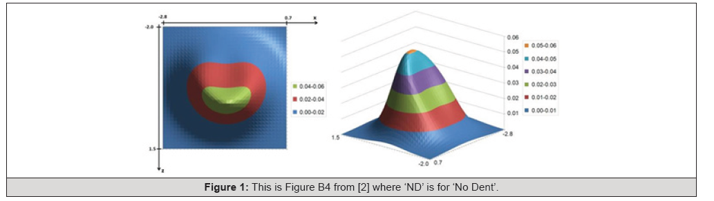
Figure 1:This is Figure B4 from [2] where ‘ND’ is for ‘No Dent’.

On our Figure 1, it is the ND case: a typical 3d-section of the 4d-graph with all three space variables involved.

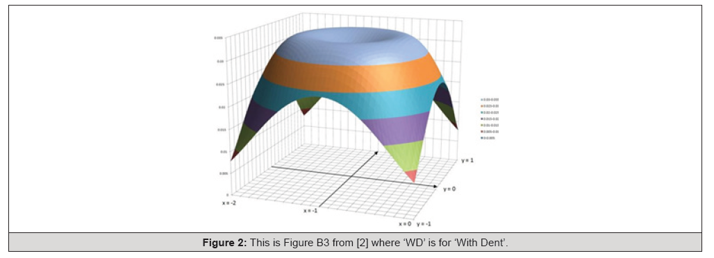
Figure 2:This is Figure B3 from [2] where ‘WD’ is for ‘With Dent’.

On our Figure 2, it is the WD-case. It is a ‘toy’ example, since only two space variables were involved. One can go (see below) beyond these two cases (ND– & WD-). As ongoing proton therapy clinical trials amass substantial statistical data, our research might be put to the test through experimental validation. Intriguingly, a different perspective could also shed light on the perplexing “reality of the wave function” enigma. Notably, a substantial contingent of experts – though perhaps not the dominant majority – align with our standpoint: that the wave function must indeed possess an objective and physical reality. This perspective opens the door to exploring correlations between our findings and distinct designs of proton vaults. Now, to get closer to the point of presenting our new findings, let us deal with the most simple ‘toy-case’. Namely, let f(x), g(x), etc., be functions of one real variable, x.

Wave Functions (an Intro ‘in Pictures’ to)

To get closer to understanding Fp, use f and g when we think of the two functions as of vectors (and interpret them as states). Let us deal with stages 1) through 5). Namely, 3) illustrates the notion of the sum f + g.

1) f(x)=1/(1 + x²)

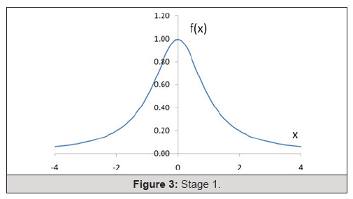
Figure 3:Stage 1.

2) g(x) = sin x

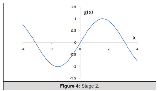
Figure 4:Stage 2.

One can think of the sum f + g as the result of (point-wise) addition of vectors on an ordinary two-dimensional (x,y)-plane R²:

3) h(x) = f(x) + g(x)

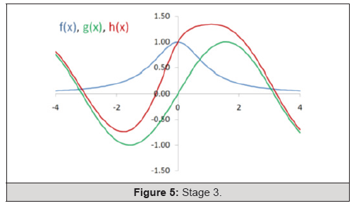
Figure 5:Stage 3.

4) F_p is an arena for different transformations. If a scaling in R² moves each (x,y) into (x/2,y/2), then a ‘vector’ f(x) goes into u(x)=1/{2(1+ 4x²)}. Recall that scaling transformations are of fundamental importance in theoretical physics. In 5) we get f - u.

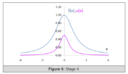
Figure 6:Stage 4.

5) Subtraction of our ‘vectors’ works as follows, here is the graph of f-u:

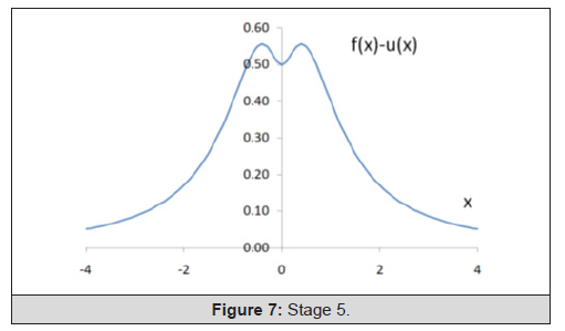
Figure 7:Stage 5.

We managed to produce an WD-element f-u. Here u was obtained from an ND-element f by scaling. This observation we are going to apply in F_p, itself.

On the Space F_p of Proton’s Wave Functions

Like in equation (6) of [2], but now we do not provide the kernel K(h,w) explicitly, the f-value at event h is the 2-dim complex vector L:

L(h) = K(h,w)v (1)

Event h (with time coordinate (x₀ and space coordinates x₁, x₂, x₃) is presented in a (well- known in theoretical physics) 2 by 2 matrix form. That is, each wave function (or state) of that type is defined by choosing a matrix w and a vector v. In [2, Theorem 4] we managed to choose w and v in such a way, that the (real) values f(h)=LL* define an ND-state f (compare to 1) – with a single point of maximum - of the prior section, and to as follows: our Figure 1. In the canonical product LL* (which is a real number) the vector L* is a complex conjugate of L.

The validity of the following statement (t there is a real parameter, while et is the coefficient of the scaling involved) is based on [3]:

Lemma 1. The image of f under scaling (with coefficient e^t) is u of type (1) but with w~ = e^-t w, v~ = e^5t/2 v.

As on our Figure 7 above, consider f – u. After calculations (they are pretty involved, see below), we put time (X₀ to 0, for a “snap shot photo”. We expect to end up with such a state F = f – u, from F_p, which has MORE THAN one points of (local or global) extrema. Here is the graphics obtained:

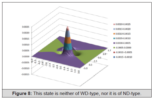
Figure 8:This state is neither of WD-type, nor it is of ND-type.

Here the scaling coefficient et was chosen as 2/3.

In the following statement (where x₀ is already set to 0), we allow an arbitrary coefficient e^t:

Lemma 2. The canonical product LL* equals to the following sum of (2) & (3), below - where by L₁, L₂, we mean the corresponding components of 2- dim vector L in (1)):

In the above, the space variables are as usual (that is: x, y, z), while other symbols are as follows:

a, b, u, v are (pretty simple) functions of x, y, z (we do not provide explicit expressions for these functions here); expressions for (real) functions A, B are quite complicated, we only indicate that they are determined by this (4):

On the basis of Lemma 2, we started to look for points of extrema for the (real) function

We have concluded that in the y=0 section of the graph of (5), there should be critical points (at this moment we do not provide them explicitly but the existence of at least one global maximum and of one local minimum follows from our graphics - above – for this very section).

Acknowledgement

None

Conflict of Interest

None

References

1. (2024) Proton Therapy –Scientific Questions and Future Direction. Monography, Intechopen ISBN 978-0-85466 88: 340-348.
2. The Proton’s Theoretical Description, Based on Wigner- Segal Approach to Elementary Particles. (Yulia Klevtsova, Alexander Levichev, Mikhail Neshchadim and Andrey Palyanov) https://www.intechopen.com/chapters/1160023
3. Jakobsen HP, Levichev AV (2022) The representation of SU (2,2) which is interpreted as describing chronometric fermions (proton, neutrino, and electron) in terms of a single composition series. Rep on Math Phys 90(1): 103-121.