Application of Bootstrap Resampling Technique to Obtain Confidence Interval for Prostate Specific Antigen (PSA) Screening Age

Introduction

Prostate cancer like lung cancer is one of the most recurrent cancer diagnosed in men universally, and the most often identified solid tumor among men in developed countries [1]. Notwithstanding a relatively high survival rates for men with prostate cancer, over 300,000 prostate cancer deaths occurred in 2012 worldwide and the universal drift of the disease is still rising. Literature has it that more than 2 million men are likely to be affected worldwide by 2040 [2,3]. Among other factors, age and family history are viewed as key risk factors for prostate cancer, black men are more volatile to the incidence of prostate cancer and death than white or Asian backgrounds [4]. The introduction of prostate-specific antigen (PSA) for prostate cancer detection in the 1990s has proved that most of cases of prostate cancer are diagnosed in men from western countries in the Americas and Europe. Prostate cancer is often dictated among men within the ages of over 40 years and most often 50 years. Research have shown that the average age confirmation age is 67 and by 70, more than half of men have at least infinites imal evidence of the disease [5]. Fortunately, prostate cancer trait generally occurs in advanced stages, making early detection worthwhile and most prostate cancer deaths usually occurs at very old age because it is usually late-maturing and are caused by something else. Two major monitoring devices for testing the prostate cancer are digital rectal examination and prostate-specific antigen (PSA) with the goal to detect clinically significant prostate cancers at a stage when intervention reduces morbidity and mortality; however, there is a growing debate on the merits and methods of screening.

It has been suggested that the use of age specific PSA reference ranges may increase the precision of PSA test since a man’s PSA level has direct relationship with age. However, age-specific reference ranges have not been generally recommended because their use may retard the detection of prostate cancer in many men. The universal use of PSA has proven controversial as the evidence for benefit as a screening test in asymptomatic men is still subject to debate, and PSA is inclined to false positives and false negatives in men with symptoms suggestive of a possible diagnosis of prostate cancer [6,7]. Moreover, PSA screening can reduce prostate cancer mortality by around 1 death prevented for every 98 men screened on a lifetime basis, but that still means for every prostate cancer death prevented by screening, 3 or 4 die from prostate cancer. In addition, PSA screening can lead to sizable over diagnosis, with approximately 5 unnecessary prostate cancer diagnosis per 100 men screened. These patients then inclined to be managed unwarrantedly, which can always cause a significant side-effect, such as incontinence and/or impotence [7]. When Prostate-specific antigen levels is less than 4ng per mL in 15 to 38 percent of men with cancer, it implies a high false-negative rate but the positive predictive value of the prostate-specific antigen test is roughly 30 %; which means that less than one in three men with an abnormal finding will have cancer on examination [8].

Such limitations of the prostate-specific antigen test have steered variations designed to improve its accuracy (e.g., age- and race-specific cutoffs, free prostate-specific antigen tests); however, none of these modifications have been widely adopted because of unsettled advantage. The major issue is that PSA monitoring may result in the detection of some cancers or diseases that ordinarily would never have bothered the patient and would never have posed a threat to his life as older men are more likely to die from heart disease and other problems than from prostate cancer. Therefore, relying too much on the test may lead to unnecessary examinations and potentially harmful treatments. Several major studies have found that PSA monitoring saves few, if any, lives. On the other hand, there is a small possibility of reducing the chance of death from prostate cancer in some cases. For men aged between 55 and 69, the choice to have a PSA examination is based on the risk factors and personal preference. However, the use of PSA-based screening for prostate cancer is discouraged for ages from 70 years and above by the United Sates Preventive Services Task Force (USPSTF). According to [8] in a meta-analysis, estimated that PSA test has a specificity of a sensitivity of 93.2 and sensitivity of 72.1. Although, such survey studies demonstrated that up to 38% of prostate cancer occur in men with PSA values less than 4ng perM1 after being diagnosed with prostate cancer [8]. The dispute over whether the advantages of the use of prostate specific antigen (PSA) exceed the treatment risks for most men has prevailed over time. In general, the current agreement is that there is no “one size fits all” guideline for who should receive prostate cancer screening and at what age. Against this backdrop was the study carried out, therefore the objective of this study is to examine the application of bootstrap resampling methods to capture the confidence interval of age of PSA screening among prostate cancer patients. The rest of the paper is organized as follows. Section 2 presents brief literature review on bootstrap techniques. Section 3 presents the material and methods. Section 4 describes the result of the analysis. Section 5 presents the summary and conclusion.

Bootstrap Method

Bootstrap and Jackknife resampling techniques are created to estimate standard errors, bias, confidence intervals, and prediction error. Works has revealed that the Bootstrap procedure is the most satisfactory for confidence interval appraisals among resampling methods. The Bootstrapping method is a resampling technique for evaluating unpredictability in which samples of size n are obtained with replacement from the original sample of size n. It is a very powerful statistical device a that can be used to evaluate the uncertainty related with a given estimator or statistical learning method and give estimates of the exactness of sample estimates of regression coefficients, fitted values and prediction of new observation and at the same time provide numerical solutions to problems whose difficulty makes the use of traditional statistical analysis unachievable and where the assumptions of regression analysis were not met [9-11].

The Bootstrap technique is also a method of calculating confidence intervals for nearly any estimate and it is theoretically simple and finding very widespread use in applied statistics and can be used to explore variations among possible models for the original dataset. The bootstrap technique enables researchers to calculate confidence intervals for any statistics regardless of the data’s underlying distribution and additional sub-samplings and replications are executed on the indigenous sample. In other words, in the beginning of the process thousands of “bootstrapped resamples” are generated from the original sampling using random sampling with replacements, after which the assigned statistic (i.e. mean, median, regression, Cronbach’s alpha coefficient, etc.) is replicated in each of these resamples. In most studies the analysts start with the population and take a sample from the population and run an analysis on that sample. Therefore, researchers may obtain thousands of estimates on the assigned statistics. Distribution of those estimates is called “bootstrap distributions”. The bootstrap distribution may be used to estimate more robust empirical confidence intervals. Bootstrapping is useful when the usual modeling methods based on assumptions about sampling distributions are untrustworthy or unavailable, for example when modeling the optimum effect of age or of dose of a treatment on performance via a quadratic relationship. The bootstrap methods can be applied to both parametric and non-parametric models, although most of the published research in the area is concerned with the non-parametric case since that is where the most instant practical gains might be expected. Often, it is used as a substitute to statistical inference based on the assumption of a parametric model when that assumption is in doubt, or where parametric inference is requires elaborate formulas or unfeasible for the estimation of standard errors [10]. In bootstrapping, the benefit of the statistic is usually calculated for more samples or each of a thousand, each of the same size as the native sample and each drawn arbitrary (with replacement) from the original sample. These values are then examined as if they came from reiteration of the study; thus, the confidence limits are given by appropriate percentiles of the values, and probabilities are given by the proportion of values falling above or below chosen magnitude thresholds. Depending on the type of the data, the method provides trustworthy values of these inferential statistics when the sample size has 20 as the least value and the number of replications is very important. Diciccio et al. [12] pinnacled the importance of using at least 2000 replications while conducting bootstrap resampling. The application of the strategy itself is explained in all tangible conditions in which the classical methods of inference operate under very limiting or impracticable hypotheses or “in asymptotic terms” [13].

Nevertheless, it is necessary to consider that Bootstrap methods raise algorithmic issues (which may be resolved with suitable IT tools only), but also interpretative difficulties regarding the reliability as well as the variability of the results. According to Banjanovic et al. [14] the uncommon use of confidence intervals is due to estimation difficulties for some statistics. Some statistics may require multi-step formulas with assumptions that might not always be viable for calculating confidence intervals. The applied bootstrap was found in 1979, Efron [15], but it was practicable to implement it without present-day computing power. One can make a probabilistic decision about the enormity of the true effect using confidence limits and probabilities as inferential statistics [16]. The method is a substitute to generating confidence limits and probabilities about the true value of the effect, and it is the only method when the sampling distribution is either not familiar or too hard to quantify. Singh [17] further stressed that a more accurate result which is far better than the traditional normal approximation can be obtained with the bootstrap estimator of the sampling distribution of a given statistic because the method is asymptotically identical to the oneterm Edgeworth expansion estimator, generally having matching convergence rate that is speedy than the normal approximation. In most modern statistical texts, the bootstrap method is suggested for estimating sampling distributions and finding standard errors, and confidence sets.

The Bootstrap Bias, the Variance, the Confidence and Percentile Interval

The mean of sampling distribution of θ ∧ often varies from θ , usually by an amount = c/ n for large n . The bootstrap bias equals,

The variance of the bootstrap from the distribution of ( ) b F θ ∧ are estimated by (Liu, 1988; Stine 1990)

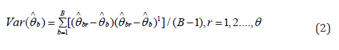
The bootstrap confidence interval by normal approach is obtained as

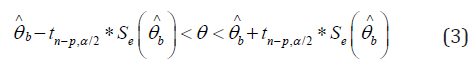
where n p, /2 t − α is the critical value of t with probability α/2 the right for n-p degrees of freedom; and Se b θ  ∧      is the standard error of the b θ ∧ . The Z-distribution values were used rather than that of t in estimating the confidence intervals when the sample size is n =30 [18]. The percentile interval which is nonparametric confidence interval can be derived from the quartiles of the sampling distribution of bootstrap of br θ ∧ . The (α/₂) % and (1-α/₂) % percentile

interval is:

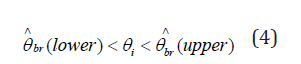
where br θ ∧ is the ordered bootstrap estimates of regression coefficient from Equation 2 or 5, lower = (α/₂)B, and upper = (1-α/₂)B.

Bias-Corrected Percentile Confidence Intervals

One issue with using the bootstrap percentile method happens when the assumption regarding the transformation to normality is violated. In such case, a confidence interval based on using the percentile method would not be relevant. In other words, the purported (supposed) confidence level is not close to the true confidence level

Material and Methods

The aim following bootstrapping is that if we don’t know what the underlying population is, then our sample is our best guess at what the underlying population is. The objective then is to extract samples from our initial sample as if we were drawing multiple samples from a population. This should work well if we are making inferences from a large sample size.

Material

The study sample comprised 100 prostate cancer patients from University of Port Harcourt Teaching Hospital. The SAS version 9.0 and SPSS statistical packages were used for the statistical analysis of the data.

Method

In our study, we bargain with the residuals resampling. The bootstrapping residuals steps are as follows:

1. We set estimate the regression coefficients from the original and compute the residuals e_i

2. For r = 1, 2,….,B, extract a n sized bootstrap sample with replacement ) e, from the residuals e_i ,and calculate the bootstrap y values

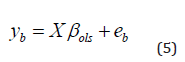
3. Estimate the regression coefficients based on equation (5), using

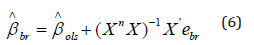
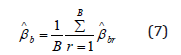
and repeat steps 2 and 3for r. Then the bootstrap estimate of the regression coefficient is:

The bootstrap bias and the variance are given below Shao et al. [19]

First, we regressed volume of capsular penetration and Gleason score on age of 100 prostate patients. Amount of capsular penetration and percent Gleason score were used as predictor variables since both are potential predictors of prostate-specific antigen (PSA) [20]. We begin with by differing the number of bootstrap samples in an uncomplicated manner, procure 50, 100, 500, 1,000, and then 10,000 bootstrap samples. We then compare the CI produced from the regression analysis by empirical bias corrected bootstrap resampling technique to those produced by the accelerated bias corrected (B_ca) method. Finally, we compute and compare the results (Tables 1 & 2). In this case, the two methods are established to occasion similar results, with differences generally at the first or second decimal place. Notice that these methods will make similar results unless the data violate parametric assumptions (e.g., data is not normal). In such cases, the bootstrapped CI will yield a better estimate because that calculation does not rely on distributional assumptions of the data [12].

Table 1: Confidence Intervals for Bias-Corrected Bootstrapped Samples.

Table 2: Confidence Intervals for Bias corrected accelerated Bootstrap (B_ca) Samples.

Results

We investigated the use of bootstrap resampling technique on confidence interval for prostate specific antigen (PSA) screening age among prostate cancer patients using OLS method with age of prostate cancer patients as a function of volume of capsular penetration and percent Gleason score as indicated above. Firstly, we considered the distribution of each variable as the tradition demands and the graphs are indicated in Figure 1. The Figure 1 shows that the data were not normally distributed and so would produce different confidence intervals. A closer look at the figure showed that all the variables were asymmetric and using such data disagrees with bootstrap distribution, in which case bias may occur. If the bootstrap distribution is non-symmetric as could be seen from the histogram above, then percentile confidence-intervals are often inappropriate. The bias-corrected and accelerated (B_Ca) bootstrap adjusts for both bias and non-normality in the bootstrap distribution. In this study therefore, we considered the bias corrected and accelerated interval method which requires no assumptions about the distribution of the data sets. For each bootstrap method of sampling, both bias-corrected and accelerated bias-corrected confidence intervals are constructed and presented in Tables 1 & 2. The OLS regression model was first fitted to data and the summary of the results is as shown in Table 1. Performing B =10,000 Bootstrap replications we obtain the results described in Table 1 and 2, where the age slope point estimate for the original sample is presented. The age, with the two predictor variables (i.e. Score and Copra) are reported in Table 1. It can be observed from the OLS regression model that the average age of prostate cancer is 53 years from the sampled data and it is significant at 5 percent level. The above table reveals that the significance of the Bootstrap increases with the sample size. The change in percentage standard deviation as a function of the number of replications is shown in Table 1. As can be seen in Figure 2, for small values of B, the confidence interval diminishes clearly and then relaxes gradually. Consequently, as B rises to 1,000, it is then balanced.

Figure 1: A histogram of the Capsular Penetration, Percent Gleason Score and Age of sampled prostate cancer patients.

Figure 2: Stability of the bias-corrected (B) 95% lower and upper bootstrap confidence intervals.

This permits us to select the number of bootstrap replications B = 1,000 with the least confidence interval 95% of the distribution. Similarly, B=1000 replications are selected to construct the bootstrap prediction intervals. The stability was achieved between 1000 and 10,000 replicates indicating the likely age interval for PSA screening. (Table 2) presents confidence intervals for bias corrected accelerated bootstrap (B_ca) samples. In Table 2, the estimator seems to be smaller across all the models and the smaller the divergence the better. The dissimilarity between confidence intervals obtained by these bootstrap methods is more pronounced when the replicates are longer. Furthermore, the most important results are the comparison between the 95% percent CI estimates. All the B_ca intervals are more realistic than the Bias corrected method, thereby improving the reliability of the estimates. The major benefit with the B_ca interval is that it corrects for bias and non-normality in the distribution of bootstrap estimates. (Figure 3) also shows divergence in confidence interval as the sample progresses. The sensitive interval for PSA screening age among prostate cancer patients was also reaffirmed between 1000 and 10,000 replicates using accelerated bias at 95% confidence interval.

Figure 3: Stability of the accelerated bias-corrected (B_ca) 95% lower and upper bootstrap confidence intervals

A closer look at the two results in terms of coverage, stipulates that B_ca intervals are “better” than B of bootstrap intervals. In other words, the B_Ca coverage is closer to the nominal value. In some cases, this may suggest that the intervals are wider or narrower than other types of bootstrap intervals. The result also agrees with the larger the sample is, the more information it carries about the parameters and this is reflected on the “precision” of the estimation. The survey reveals that confidence intervals constructed under B_ca has better coverage ability, tighter and a narrower width which is desired for any coverage probabilities compared to bias-corrected. A look at Table 3 shows that between 500 and 10,000 replicates, both biased correlated and accelerated biased correlated bootstrap resampling methods exhibited the same bias value (i.e. -0.309,- 0.139 and -0.24) which further confirmed the stability in age of sampled patients. However, the best interval occurred at 1000 since it has the least confidence interval. An interesting finding of this study is the convergence of both methods which is indicates after 1000 replicates were the least confidence interval was attained. Since confidence level refers to the long-term success rate of the method, that is, how often this type of interval will capture the parameter of interest. A specific confidence interval gives a range of plausible values for the parameter of interest. This suggests that the appropriate age of prostate cancer screening is from 41 years and above with an interval repeat of 4 years.

Conclusion

The use of bootstrap method paves a way of reducing bias and getting the standard errors in cases where the standard techniques might be expectedly inappropriate. Accordingly, in practice, we recommend the use of the bootstrap method in estimating the variance and constructing confidence intervals related with nonparametric regression estimator. The study reveals that starting PSA screening age among prostate cancer patients should be from 41 years, with repeats at 45 (i.e.an interval repeat of 4 years) will help detect those extremely aggressive cancers that tend to occur in men in their early fifties with remarkably low serum PSA and this findings is in line with EAU [7], but with high risk poorly differentiated tumors that hardly express PSA. Change in PSA levels between 40 and 50 will raise suspicion of these deadly prostate cancers.” This study has shown that use of bootstrap confidence interval could be used to improve the accuracy of PSA-based prostate cancer screening.

References

• Merriel SWD, Funston G, Hamilton W (2018) Prostate Cancer in Primary Care. Adv Ther 35(9): 1285-1294.
• Bray F, Ferlay J, Soerjomataram I, Siegel RL, Torre LA, et al. (2018) Global cancer statistics 2018 GLOBOCAN estimates of incidence and mortality worldwide for 36 cancers in 185 countries. CA Cancer J Clin 68(6): 394424.
• (2015) NICE. Suspected cancer: recognition and referral. p. 1-95.
• Ferlay J, Soerjomataram I, Ervik M (2018) GLOBOCAN 2012 v1.0, Cancer Incidence and Mortality Worldwide: IARC Cancer Base No. 11. International Agency for Research on Cancer, Lyon.
• Penn State Health Milton S Hershey Medical Center.
• Grossman DC, Curry SJ, Owens DK, et al. (2018) Screening for prostate cancer: US Preventive services task force recommendation statement. JAMA 319(18): 1901-1913.
• European Association of Urology (2015) Prostate cancer screening under age of 55 may be of limited value. Science Daily.
• Wilbur J, Roy J, Lucille A (2008) Prostate Cancer Screening: The Continuing Controversy. American Family Physician 78(12): 1378 -1384.
• Efron B (1981) Nonparametric estimates of standard error: the jackknife, the bootstrap and other methods. Biometrika 68(3): 589-599.
• Efron B, Tibshirani R (1986) Bootstrap methods for standard errors, confidence intervals and other measures of statistical accuracy. Stat Sci 1: 54-75.
• James G, Witten D, Hastie T, Tibshirani R (2014) An introduction to statistical learning: with applications in R. Springer, USA
• Diciccio TJ, Efron B (1996) Bootstrap confidence intervals (with Discussion) Statistical Science 11: 189-228.
• Giudice VD, Salvo F, De Paola P (2018) Resampling Techniques for Real Estate Appraisals: Testing the Bootstrap Approach. Sustainability 10(9): 3085
• Banjanovic ES, Osborne JW (2016) Confidence Intervals for Effect Sizes: Applying Bootstrap Resampling. Practical Assessment and Research Evaluation 21(5).
• Efron B (1987) Better bootstrap confidence intervals (with discussions). Jour Amer Stat. Assoc 82: 171-200.
• Hopkins WG (2012) Bootstrapping Inferential Statistics with a Spreadsheet. Sportscience 16: 12-15
• Singh K (1981) On Asymptotic accuracy of Efron’s bootstrap. Ann Stat 9: 1187-1195.
• Di Ciccio TJ, Tibshirani R (1987) Bootstrap confidence intervals and bootstrap approximations. J Am Statist Assoc. 82: 163-170.
• Shao J, Tu D (1995) The Jackknife and Bootstrap. Springer-Verlag, New York, USA.
• Stamey TA, JN Kabalin, JE McNeal, IM Johnstone, F Freiha, et al. (1989) Prostate specific antigen in the diagnosis and treatment of adenocarcinoma of the prostate. II. Radical prostatectomy treated patients. Journal of Urology 141: 1076-1083.