Research Article 
![]() Creative Commons, CC-BY
Creative Commons, CC-BY
Hybrid Species and Closed-Form Solutions of the Lotka-Volterra Equations
*Corresponding author: Jean-Luc Boulnois, Babson College, Babson Park, Wellesley, Massachusetts 02457, USA, Email: jlboulnois@msn.com
Received: April 12, 2023; Published: April 28, 2023
DOI: 10.34297/AJBSR.2023.18.002503
Abstract
The classical Lotka-Volterra system of two coupled non-linear ordinary differential equations is expressed in terms of a single positive coupling parameter λ , ratio of the respective natural growth and decay rates of the prey and predator populations. “Hybrid-species” are introduced resulting in a novel λ − invariant Hamiltonian of two coupled first-order ODE albeit with one being linear; a new exact, closed-form, single quadrature solution valid for any value of λ and the system’s energy is derived. In the particular case λ = 1 the ODE system partially uncouples and new, exact, closed-form time-dependent solutions are derived for each individual species. In the case λ ≠ 1 an accurate practical approximation uncoupling the non-linear system is proposed; solutions are provided in terms of explicit quadratures together with analytical high energy asymptotic solutions. A novel, exact, closed-form expression of the system’s oscillation period valid for any value of λ and orbital energy is derived; two fundamental properties of the period are established; for λ = 1 the period is expressed in terms of a universal energy function and shown to be the shortest.
Keywords: Single coupling parameter; Quadrature solutions; Asymptotic solutions; Period
Introduction
This paper is a revised version of two articles which were first published on arXiv and subsequently merged [1,2].
The historic Predator-Prey problem, also known as the Lotka- Volterra (“LV”) system of two coupled first-order nonlinear differential equations has first been investigated in ecological and chemical systems [3,4]. This idealized model describes the competition of two isolated coexisting species: a ‘prey population’ evolves while feeding from an infinitely large resource supply, whereas ‘predators’ interact by exclusively feeding on preys, either through direct predation or as parasites. This two-species model has further been generalized to interactions between multiple coexisting species in biological mathematics [5], ecology [6], virus propagation [7], and also in molecular vibration-vibration energy transfers [8]. As a result of their competition, the respective populations exhibit undamped oscillations as a function of time with a period which depends on the species interaction rates together with the system’s energy.
Normalized Equations and Single Coupling Parameter
The classical LV model is based on four time-independent, pos itive, and constant rates with two representing species self-inter action, i.e. natural exponential growth rate α and decay rate δ per individual of the respective prey and predator populations, and two others characterizing inter-species interaction.
Without any loss of generality, the LV system of two coupled
first order ordinary differential equations (ODE) can be simplified
by simultaneously scaling the predator and prey populations together
with time through a dimensionless time t based on the factor
 . The system is shown to only depend on a single positive
coupling parameter λ , ratio of the respective growth and decay
rates of each species taken separately, defined as
. The system is shown to only depend on a single positive
coupling parameter λ , ratio of the respective growth and decay
rates of each species taken separately, defined as

Let u (t ) ≥ 0 and v (t) ≥ 0 be the respective instantaneous populations of preys and predators assumed to be continuous functions of time t : upon inserting λ as defined in (1) into the standard LV two-equation system, a normalized form is obtained as a set of two coupled first-order autonomous nonlinear ODEs solely depending on this single coupling ratio λ , [1].
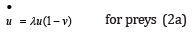
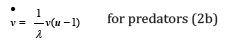
The “dot” in u  and v
and v  indicates a derivative with respect to the time
t : in the sudden absence of coupling between species, the prey
population would grow at an exponential rate λ while predators
would similarly decay at an inverse rate −1 / λ from their respective
positive initial values.
indicates a derivative with respect to the time
t : in the sudden absence of coupling between species, the prey
population would grow at an exponential rate λ while predators
would similarly decay at an inverse rate −1 / λ from their respective
positive initial values.
Remarkably, the normalized ODE system (2) is invariant in the transformation u → v together with λ → −1 / λ : this fundamental property, subsequently referred to as “λ − invariant ”, is extensively used throughout to considerably simplify the LV problem analysis.
Numerous solutions of the non-linear system (2) using a variety of techniques have been proposed including trigonometric series [9], mathematical transformations [10], Taylor series expansions [11], perturbation techniques [12,13], numeric-analytic techniques [14] and Lambert W-functions [15,16]. Also, an exact solution has previously been derived in the special case when the prey growth rate and predator decay rate are identical in magnitude, but with opposite signs, i.e. α = −δ , a condition which precludes population oscillation. The basic system (2) is non-trivial and analytical closed form solutions are unknown.
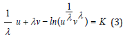
Since the original publications [3,4], the system (2) has been known to possess a dynamical invariant or “constant of motion K” expressed here in λ − invariant form
In the following sections, through a functional Hamiltonian transformation combined with a suitable linear change of variables, a novel λ − invariant Hamiltonian based on new “hybrid-species” reduces the system (2) to a new set of two coupled first-order ODEs with one being linear. As a result, a new, exact analytical solution is derived for one hybrid-species in terms of a simple quadrature: we then proceed with an original method to uncouple the system and derive complete, closed-form quadrature solutions of the LV problem. In the case λ = 1 , an exact analytical solution of the LV system for each individual prey and predator species u (t) and v (t) is derived as a function of time. The population oscillation period is further expressed in terms of a unique energy function and two fundamental properties of the period are established.
Solutions with Hybrid Predator-Prey Species
The logarithmic functional transformation originally introduced
by Kerner [17] reduces the normalized LV system (2) to a
Hamiltonian form: the coupling between the respective species is
modified through a change of variables y and x ∈  according to
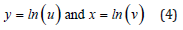
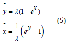
The LV system (2) for the respective “logarithmic” prey-like and predator-like species y(t) and x(t) becomes
Similarly to Eq. (3) this λ − invariant system (5) admits a primary conservation integral H expressed as the linear combination of two positive convex functions
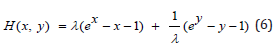
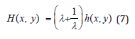
As already established [18,19], H(x, y) is the Hamiltonian of the conservative LV system since Eqs. (5) satisfy Hamilton’s equations with x as the coordinate conjugate to the canonical momentum y. Equation (6) expresses the conservative coupling between species x(t) and y(t) : it is further rendered λ − invariant by introducing a scaled Hamiltonian h(x, y) with total constant positive energy simply labeled h , according to
We introduce a λ − invariant linear first-order ODE between the species x(t) and y(t) by further combining the system (5) with (6) and (7)

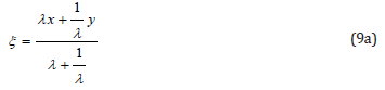
Equation (8) suggests introducing a λ − invariant linear transformation of the set {x (t), y (t)} to a new set {ξ (t),η (t)} representing the symbiotic coupling between ”hybrid predator-prey species”

The original Hamiltonian (6) together with (7) and the linear transformation (9) then becomes
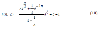
Here h(η ,ξ ) is a new Hamiltonian for the coordinate η and its conjugate momentum ξ . Notice that for small amplitudes, h(η ,ξ ) identically reduces to the Hamiltonian of a harmonic oscillator. Upon further introducing the following λ − invariant G- function

the conservation relationship (10) between the conjugate functions η(t n(t) and ξ (t) is recast into a compact form which provides a natural separation of variables

In the following we define a useful compact auxiliary function U(ξ ) ≥ 1 appearing throughout as

Even though still nonlinear, the fundamental conservation relationship (12) partially uncouples the ξ (t) -function from the n(t) -function, resulting in three essential G -function properties:
I. The system’s energy h ≥ 0 is explicitly associated with the function U (ξ ) only;
II. The positive function Gλ (η ) is a generalized hyperbolic cosine
function that reaches its minimum Gλ = 1 at η = 0 for any
value of λ : hence its inverse function  exists, and, for any
value of λ , Eq. (12) admits two respective positive and negative
roots η ± (ξ ,λ ) functions of ξ only satisfying
exists, and, for any
value of λ , Eq. (12) admits two respective positive and negative
roots η ± (ξ ,λ ) functions of ξ only satisfying

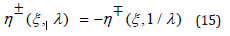
III. Since the η-function is associated with the coupling ratio λ only, λ − invariance of the G-function (11) implies that, for a given λ , any positive solution η + (ξ ,λ ) is directly derived from the negative solution associated with the ratio 1 / λ , and reciprocally
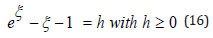
From Eq. (13) the hybrid-species population ξ (t) thus oscillates between the λ − independent respective negative and positive roots ξ − (h) and ξ + (h) , solutions of the equation U (ξ ) = 1, solely dependent on the system’s energy h as displayed in Table 1 for several increasing values of h

Table 1: Roots of eξ −ξ −1 = h as a function of the energy h from Eq. (16).
For any value of the energy h , in the ξ −η plane Eq. (12)
represents a closed- orbit loop consisting of two branches
η + (ξ ,λ ) and η − (ξ , λ ) around the fixed point (0, 0) . This mapping
is bounded by the roots ξ − (h) and ξ + (h) on the horizontal
axis; since U (ξ ) admits a maximum eh located at ξ = −h , it is also
bounded vertically by the two respective positive and negative
roots solutions of the equation 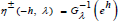 . An orbit is
displayed on Figure 1 for an energy h = 2 and two inverse coupling
parameters λ = 2 and λ = 1 / 2 . Per Eq. (15), the respective
branches associated with the λ and 1 / λ -mappings are readily observed
to be symmetric with respect to the η = 0 axis.
. An orbit is
displayed on Figure 1 for an energy h = 2 and two inverse coupling
parameters λ = 2 and λ = 1 / 2 . Per Eq. (15), the respective
branches associated with the λ and 1 / λ -mappings are readily observed
to be symmetric with respect to the η = 0 axis.
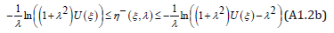
Except when λ = 1 , algebraic solutions of Eq. (14) may generally not be obtained directly. However, for any value ξ ∈[ξ − (h),ξ + (h)] the two roots η ± (ξ , λ ) of Eq. (14) may be obtained numerically through a standard ”Newton-Raphson” algorithm. Appendix 1 establishes that each root admits lower and upper bounds for any value of U (ξ ) , thereby ensuring algorithm convergence.
Lastly, upon inserting the linear transformation (9) into the modified LV system (5), or equivalently using the standard Hamilton equations with Eq. (10), a new semi-linear system of coupled 1st order ODEs is obtained

Figure 1:ξ −η Mapping for λ = 2 and λ = 1 / 2 , and energy h = 2 .
The solution of the system (17), in which  is the derivative
 , represents the time-evolution of the hybrid-species
n(t) and ξ (t) , albeit due to the linear transformation (9), the first
coupled equation (17a) becomes linear as expected. Remarkably, as
a result of this hybrid-species transformation, the linearity considerably
simplifies the solution of the system (17). The exact solution
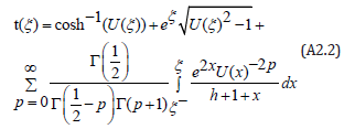
of the LV problem is derived by integration of (17a) as a simple
closed-form quadrature for t(ξ ) : upon using the initial conditions
η0 = 0 and ξ0 = ξ ± (h) when t = 0 , the exact LV solution corresponding
to the respective negative and positive branches η − (ξ , λ ) and
η + (ξ , λ ) becomes
, represents the time-evolution of the hybrid-species
n(t) and ξ (t) , albeit due to the linear transformation (9), the first
coupled equation (17a) becomes linear as expected. Remarkably, as
a result of this hybrid-species transformation, the linearity considerably
simplifies the solution of the system (17). The exact solution
of the LV problem is derived by integration of (17a) as a simple
closed-form quadrature for t(ξ ) : upon using the initial conditions
η0 = 0 and ξ0 = ξ ± (h) when t = 0 , the exact LV solution corresponding
to the respective negative and positive branches η − (ξ , λ ) and
η + (ξ , λ ) becomes
This quadrature is not divergent at x = − h , since the differential
dη in Eq. (14) contains the factor  in the
numerator. Upon using the same initial conditions, the solution
(18) is expressed in terms of the function η ± (ξ , λ )
itself through
a standard integration by parts in which the singularity at ξ = −h
is further eliminated by adding and subtracting the expression
in the
numerator. Upon using the same initial conditions, the solution
(18) is expressed in terms of the function η ± (ξ , λ )
itself through
a standard integration by parts in which the singularity at ξ = −h
is further eliminated by adding and subtracting the expression
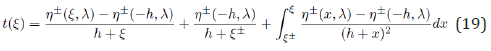
 in the integral. The final, exact, closed-form, regular solution
of the entire LV problem for any value of the coupling ratio λ
and/or of the orbital energy h is explicitly expressed as a quadrature
over each of the two branches η ± (ξ , λ ) solutions of (14)
in the integral. The final, exact, closed-form, regular solution
of the entire LV problem for any value of the coupling ratio λ
and/or of the orbital energy h is explicitly expressed as a quadrature
over each of the two branches η ± (ξ , λ ) solutions of (14)
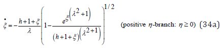
This exact solution is further analyzed in the following section. Numerical solutions for ξ (t) and η (t) are also obtained by integrating Eqs. (17) using a standard fourth-order Runge-Kutta (RK4) method as presented in Figure 2 for values of h and λ exactly identical to those of Figure 1, together with the above initial conditions η0 and ξ0 . The function ξ (t) is observed to principally depend on two time constants: a quasi-exponential increase at a rate of order λ followed by an exponential decrease at a rate −1 / λ : from λ − invariance (15) the two functions ξ (t) respectively corresponding to λ = 2 and its inverse λ = 1 / 2 are mirrors of each other; so are the functions η (t) , but with the change η → −η
For the general case λ ≠ 1, upon explicitly relating Gλ (η ) to its
derivative  and expressing the latter as an analytical function
of ξ only through (12), an ap- proximate yet accurate ODE for
ξ (t) is proposed below.
and expressing the latter as an analytical function
of ξ only through (12), an ap- proximate yet accurate ODE for
ξ (t) is proposed below.
Case λ = 1 . The LV problem is solved exactly in the particular case λ = 1 , [2]. The G-function (11) (omitting the index for simplicity) reduces to the hyperbolic cosine function and the energy conservation equation (12) becomes
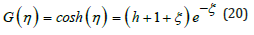

Figure 2: Solutions for ξ (t) and η (t) as a function of time t with λ = 2 and energy h = 2 : numerical integration of Eq. (17) by RK4.
The resulting ξ –η closed-orbit mapping is symmetric with two branches η ± (ξ ) explicitly expressed in terms of the inverse hyperbolic cosine function
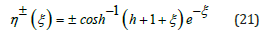
Equation (21) again establishes the symbiotic coupling between the hybrid species η and ξ . Evidently, in this λ = 1 case, the explicit relationship between G (η ) and its derivative G′(η ) is
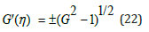
Upon inserting (22) together with (20) into (17b) the nonlinear LV system (17) completely uncouples: it consists in the 1st order linear ODE (17a) together with a 1st order nonlinear autonomous ODE for the species ξ population

The linear equation (23a) is directly solved by inserting η (ξ ) from (21) into the solution (19). Together with U (ξ ) defined in (13), the exact, closed-form analytic solution on the interval ξ − ≤ ξ ≤ ξ + is thus expressed as a simple quadrature in terms of elementary functions
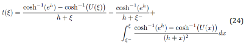
By applying l’Hoˆpital’s rule, it is readily verified that the integrand in (24) is regular at ξ = −h . Figure 3 presents the ξ (t) − solution obtained by numerical RK4 integration of (24) for an energy h = 2 with initial condition ξ (0) =ξ − (h) . The growth and decay phases of the function ξ (t) are observed to be symmetric relative to the half-period t* when ξ (t∗) =ξ +(h) . The LV solution is finalized for the two branches η ± (t) by inserting ξ (t) derived above into Eq. (21).
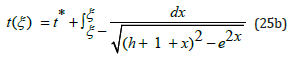
Alternatively, over the respective intervals ξ − ≤ξ (t) ≤ξ + and
 corresponding to the growth and decay phases of
ξ (t ) , an expression for t (ξ )
is readily obtained by performing the
integration with the respective positive root (growth phase) and
negative root (decay phase) of the autonomous Eq.(23b), yielding
the following quadrature solution which only depends on the energy
h
corresponding to the growth and decay phases of
ξ (t ) , an expression for t (ξ )
is readily obtained by performing the
integration with the respective positive root (growth phase) and
negative root (decay phase) of the autonomous Eq.(23b), yielding
the following quadrature solution which only depends on the energy
h
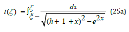
Even though the ξ (t) hybrid species population is not explicitly
expressed as a function of time t, the function t (ξ ) being monotonic
and continuous on each respective integration interval, its inverse
function  defined by ξ (t ) = t−1(ξ ) , exists and is unique,
monotonic, and continuous on each interval. At the respective limits
ξ − (h) and ξ + (h) the integrand of (25) has a weak singularity of the
square root type but is strictly continuous over the interval and the
integral is convergent. It is readily verified that integrating (24) by
parts identically results in solution (25).
defined by ξ (t ) = t−1(ξ ) , exists and is unique,
monotonic, and continuous on each interval. At the respective limits
ξ − (h) and ξ + (h) the integrand of (25) has a weak singularity of the
square root type but is strictly continuous over the interval and the
integral is convergent. It is readily verified that integrating (24) by
parts identically results in solution (25).

Figure 3: Solutions for ξ (t) and η (t) as a function of time t obtained by numerical integration of the quadrature solution Eq. (23b) with λ = 1 and energy h = 2 .
Together with (21), the exact solution (25) for ξ (t) over the respective intervals ξ − ≤ ξ ≤ ξ + and ξ + ≥ ξ ≥ ξ − constitutes the final solution of the LV problem for the “hybrid species” in the special λ = 1 case considered here.
The solution (25) is similar in form to one derived by Evans and Findley (Eq. (17) in [10]); however, the above integral expression lends itself to simpler analytical or numerical integration. An exact expression for (25) is further proposed in Appendix 1 in terms of exponential integral functions.
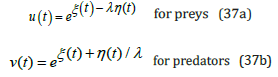
Exact Solutions for the Prey and Predator Species Populations. In this λ = 1 case, exact solutions for the time evolution of the prey and predator populations are derived by inserting the respective hybrid-species populations ξ (t) and η (t) obtained from Eqs. (25) and (21) into the original definitions (4) and (9). This results in two uncoupled solutions for the individual populations u (t) and v(t) of the prey and predator species.
Over the growth and decay phases of the symmetric ξ (t) function, these exact un- coupled analytical solutions for the respective prey and predator populations are expressed as follows
 growth phase
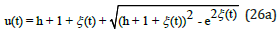 for preys
 for predators with
  derived from (25a) together with
  .
.
 decay phase
 for preys
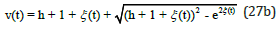 for predators
with  derived from (25b) together with
Figure 4 displays the exact uncoupled analytical solutions for the time evolution of the preys u (t) and the predators v(t) when their respective growth and decay rates are equal in magnitude, and when the system’s energy is h = 2 .

Figure 4: Exact analytical solutions for u (t ) and v (t ) as a function of time t obtained from Eqs. (26) and (27) with energy h = 2 .
It is observed that the prey population u (t)
exhibits an initial
growth at rate significantly slower than its own fast decay rate with
the opposite for predators; also the peak population of the preys occurs
when the population is mature, i.e. when the predator population
is small (v = 1) , and vice-versa.
Case λ ≠ 1. In the general case when λ ≠ 1 the relationship between
and its derivative G'λ η
is obtained by observing that
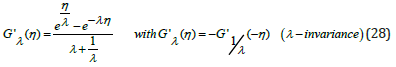
Upon eliminating η between Eqs. (11) and (28), an implicit non-linear 1st order ODE relating G to its derivative Gj is derived (for clarity the index λ is omitted in the remainder of this section)
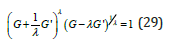
Equation (29) is completely invariant in the change λ →−1/λ , or equivalently changing λ →1/λ together with G'→ −G' . As a result, similarly to Eq. (22), in the G −G' phase space, Eq. (29) represents the positive and negative branches of a “skewed” hyperbola with orthogonal asymptotes, respectively G' = G /λ and G' = −λG , and a vertex G' = 0 located at G' =1. For any value of the coupling parameter λ , the function G'(η ) reaches its extremes at the two roots of G(η ) = eh . Also, as expected, in the case λ =1 Eq. (29) identically reduces to (22).
Being implicit, (29) can generally not be solved for G' as a function of G by standard algebraic techniques. A practical yet accurate approximation for the function G'(G) predicated on Eq. (22), which uncouples the system, is proposed below.
For the positive branch G' ≥ 0 , for large G the function G' is asymptotic to G' = G /λ : Eq. (29) is recast as
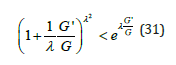
Furthermore, the factor in parenthesis in the denominator always satisfies the following inequality
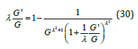
Upon approximating this factor by its exponential limit, Eq. (30) becomes

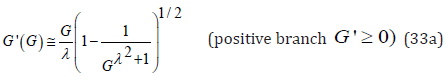
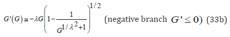
Since the G-function is bounded by eh , a Taylor expansion of the exponential factor to first order yields an explicit approximation for the two branches of G'(G) . Notice that the negative branch G' ≤ 0 is directly obtained by λ − invariance applied to the equation representing the positive branch G, ≥ 0 .
Remarkably, the above approximate function G'(G) satisfies the following three basic properties identical to those of an exact numerical solution of Eq. (29):
1. At its vertex, when G = 1, the function G'(G) reaches G' = 0 ,
2. For G >> 1, as expected, the positive branch of the function G'(G) is asymptotic to G' = G /λ whereas the negative branch is asymptotic to G' = −λG ,
3. For λ = 1, G'(G) reduces to the exact predicate expression (22).
Thus, in the G −G' phase space, the explicit expressions (33) represent approximate positive and negative branches of the “skewed” hyperbola defined by Eq. (29) with the same orthogonal asymptotes. Upon comparing graphic representations of the explicit expressions (33) to the exact numerical solution of (29) for the implicit function G'(G) it is found that the agreement is quite reasonable particularly for the positive G'(G) -branch when λ ≥1, and conversely for the negative branch when λ ≤1. This is understandable in light of the above first two properties of (33). As λ →1 the approximation (33) approaches the exact solution (22); for λ 1 the graph of (33) exhibits two branches tightly bounded by their respective orthogonal asymptotes with the accuracy of this approximation increasing with increasing λ .
As intended, approximation (33) effectively uncouples the system (17) by explicitly removing the dependence on η in the original ODE (17b): upon inserting the con- servation Eq. (12) into (33), Eq. (17b) is replaced by a pair of two λ − invariant 1st order nonlinear ODEs for the hybrid species population ξ (t)

Evidently, for λ = 1 the two branches of (23b) are recovered. Even though ξ (t) is not explicitly expressed as a function of time t, the arbitrary λ ≠ 1 problem has thus been reduced to a pair of simple quadratures for the function ξ (t) . As already stated, the function ξ (t) oscillates between the λ-independent respective roots ξ − (h) and ξ + (h) solutions of Eq. (16). The process for solving Eq. (34) is identical to that of Eq. (23b): upon again choosing the time origin t = 0 when ( ) 0 ξ =ξ − h , a complete period is obtained by integration over the corresponding negative η − branch in (34b) until ξ (t) reaches ξ + (h) , followed by an integration over the positive η − branch (34a) until ξ − (h) is reached
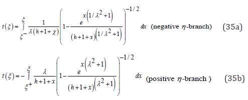
The function t (ξ ) being monotonic and continuous on the respective integration intervals ξ − ≤ξ ≤ξ + and ξ + ≥ξ ≥ξ − its inverse function ξ (t) exists and is unique, monotonic, and continuous on each interval. The LV problem is then completed for the function η (t) by directly integrating the linear Eq. (17a) through standard numerical techniques.
To assess the accuracy of the uncoupled approximate solutions (34), a comparison is made with the exact numerical solutions of the original coupled LV system (17). Upon using the respective values λ = 2 and h = 2 identical to those of Figure 2 for the coupling ratio and system energy, Figure 5 presents the comparison between the functions ξ (t) and η (t) respectively obtained by numerically integrating (34) and (17) simultaneously through a standard 4th order RK4 method. From the figure it is observed that the ODEs (34) provide a reasonably accurate solution for both functions ξ (t) and η (t) over an entire period, yet, when λ >1, with an underestimation of the time taken to reach ξ + (h) compensated by an overestimation of the time to reach ξ − (h) . As expected, the accuracy of the solutions obtained with approximations (34) increases with increasing λ .
From Figure 5, regardless of the value of λ , the hybrid species population ξ (t) oscillates with exponential-like growth and decay phases with an amplitude determined by its energy-dependent interval ξ + (h) −ξ − (h) .
Remarkably, in the high energy limit h 1, upon keeping the leading asymptotic term in (34), the asymptotic behavior of the LV system becomes modeled as a system of two coupled linear 1st order ODEs for each hybrid species. In this asymptotic limit, together with the linear ODE (17a) for η (t) , the system admits trivial exponential solutions remarkably representative of the exact solutions of (17). For example, the asymptotic solutions h >> 1 for the growth phase (ξ − ≤ξ ≤ξ + ) simply are
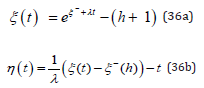

Figure 5: Solutions for ξ (t) and η (t) as a function of time t with λ = 2 and energy h = 2 ; comparison between RK4 numerical integration of Eq. (17) and Eq. (34).
The asymptotic decay phase solutions for ξ (t) and η (t) are obtained by λ − invariance , namely λ → −1/λ together with ξ − (h)→ ξ + (h) .
Lastly, as done with the exact solutions (26) and (27) when λ =1, upon inserting the hybrid-species populations ξ (t) and η (t) derived from Eqs. (34) together with the transformation (9) into the prey and predator species definition (4), the respective standard solutions for the original populations u (t) and v(t) are fully recovered when λ ≠ 1
Oscillation Period of the LV System
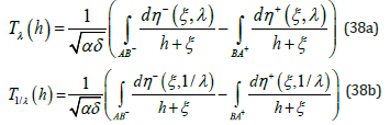
The unique λ − invariance property of η ± (ξ ,λ ) in (15) directly enables to establish two fundamental properties of the LV system period [1]. Consider the double mapping of Figure 1 and follow in a counter clockwise direction the two branches AB− and BA+ corresponding to the respective branches η (ξ ,λ ) − and η + (ξ ,λ ) : the negative branch AB− starts at ξ − (h) and ends at ξ + (h) and conversely for the positive BA+ branch. Upon integrating (18) over the ξ − variable and recalling the earlier dimensionless time definition, the oscillation period T (h) λ associated with the λ -mapping is directly obtained as a quadrature over these two branches in (38a) in which the negative sign for the second integral reflects integration from ξ + to ξ − . Similarly, for the 1/λ -mapping the oscillation period is expressed as (38b)
Upon recalling the λ − invariance property of Eq. (15), substitution into (38b) establishes that:
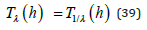
Theorem 1. For any value of the positive orbital energy h, the LV system oscillation periods respectively corresponding to the coupling ratio λ and its inverse 1/λ are equal.
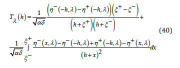
Consequently, an exact, closed-form, regular expression for the nonlinear LV system oscillation period, valid for any value of the coupling ratio λ and any value of the orbital energy h, is directly derived from (38a) as a single integral over the two branches η ± (ξ , λ)
In Appendix 1, for any  the interval
  is shown to be a positive increasing function of λ when λ ≥1(and decreasing when 0 < λ ≤1) admitting respective
lower and upper bounds, both of which are minimal when λ = 1
. Together with Eq. (40) this establishes:
is shown to be a positive increasing function of λ when λ ≥1(and decreasing when 0 < λ ≤1) admitting respective
lower and upper bounds, both of which are minimal when λ = 1
. Together with Eq. (40) this establishes:
Theorem 2. For any value of the positive orbital energy h , the LV system oscillation period T (h) λ is an increasing function of λ for λ ≥1 (decreasing for 0 < λ ≤1) and the period is shortest for λ =1.
In the particular case when λ =1, the exact LV system period
 is uniquely expressed in terms of a universal energy function

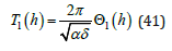
The LV energy function Θ1 (h) introduced in is defined by integrating (25a) over the entire ξ − interval
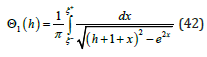
At small orbital energy (h <<1)where ξ ± (h) = ± 2h , the function Θ1 (h) is directly expressed in terms of the complete elliptic integral of the first kind K (k ) with its modulus k
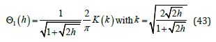
A standard series expansion for K (k ) yields
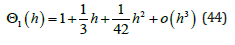
For small oscillation amplitudes, the integral (42) becomes
independent of the energy h and is exactly equal to π , hence
Θ1 (h) = 1; the LV system becomes that of two coupled harmonic oscillators
for which the period T(h) solely depends on the pulsation
 , as already established [3,20].
At high orbital energy (h >>1), the contribution from the exponential term in (42) becomes negligible since ξ < 0 over most of the integration interval except when ξ approaches ξ + (h) : since by definition ξ (t) ≥ξ − (h) , approximating the exponential term by its lowest value e2ξ −(h) and performing the integration yields a useful asymptotic expression for Θ(h)

When λ ≠ 1 the exact LV oscillation period Tλ (h)
is obtained
by numerically solving the ODE system (17) as done for Figure
2. Similarly to Eq. (41), for each value of the coupling ratio λ , the
period T λ (h)
is then uniquely expressed in terms of a universal LV
energy functions 
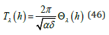
As shown on Figure 6 and consistent with Theorem 2, for any value of the coupling parameter λ , each function Θλ(h), and by extension T (h) λ , is a monotonically increasing function of the energy- dependent amplitude ξ + (h) −ξ − (h) of the ξ (t) function only [20]. Also displayed is the asymptotic approximation (45) which is practically indistinguishable from the exact function Θ1(h) for h ≥ 4 .

Figure 6: Energy function Θλ(h) for λ =1, 2,3, 4,5 and asymptotic approximation for λ =1.
In this general λ ≠ 1 case, an asymptotic formula for the LV
system oscillation period Tλ (h)
valid at high energy (h >>1)
is
obtained from the asymptotic solutions (36). The contribution
 of the exponential growth phase of ξ (t)
to the period is
readily obtained from (36b) since η (t) = 0
when ξ (t) reaches its
maximum
of the exponential growth phase of ξ (t)
to the period is
readily obtained from (36b) since η (t) = 0
when ξ (t) reaches its
maximum  ; the contribution
  of the decay phase is obtained
by λ − invariance . As a result the high energy (h >>1) asymptotic
expression for the LV system period T (h) λ simply becomes
proportional to the sum of the ξ (t ) −
function growth and decay
rates, λ and 1/λ , respectively
of the decay phase is obtained
by λ − invariance . As a result the high energy (h >>1) asymptotic
expression for the LV system period T (h) λ simply becomes
proportional to the sum of the ξ (t ) −
function growth and decay
rates, λ and 1/λ , respectively
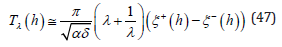
This asymptotic formula which separately factorizes the LV system coupling from the λ − independent energy contribution satisfies both Theorem 1 and Theorem 2 since it is minimal when λ =1.
Upon comparing the methods of Volterra [3], Hsu [21], Waldvogel [20], and Rothe [22], Shih demonstrated that all of these integral representations of the period of the two-species LV system are equivalent to his own solution in terms of a sum of convolution integrals [15]. Subsequent approximations of the LV system period in terms of power series [23] or perturbation expansions [24] have also been published. In Appendix 3, following the derivation of Rothe [22], we show that the Hamiltonian (10) based on hybrid-species populations defined in (9) provides a ”state sum” identical to that of Rothe thereby establishing direct equivalence between our LV oscillator period and Rothe’s convolution integral.
Conclusion
The coupled 1st order non-linear ODE system for the LV problem of two interacting prey and predator species has been analyzed in terms of a single positive coupling parameter λ , ratio of the relative growth/decay rates of each species taken independently. Based on a standard functional transformation introducing” hybrid-species populations”, a novel λ − invariant set of two 1st order ODEs is obtained with one being linear. As a result, an exact, closed-form quadrature solution of the LV problem is derived for any value of the coupling ratio λ and any value of the system’s energy (19).
In the λ =1 case, the LV problem partially uncouples and an exact explicit closed form solution is derived in terms of the system’s orbital energy h as a simple quadrature for the time evolution of the hybrid-species population ξ (t) ; the other hybrid species’ solution η (t) is explicitly expressed in terms of the former (Eqs. (25) and (21)). As a result, exact uncoupled analytical solutions for each of the original prey and predator populations u (t ) and v (t ) are derived as a function of time.
In the λ ≠ 1 case, a λ − invariant accurate practical approximation is derived that explicitly uncouples the LV system and provides a closed-form solution in terms of a single quadrature for one of the hybrid-species populations. Remarkably, at high orbital energies (h >>1), the original coupled non-linear LV ODE system totally uncouples and becomes entirely linear admitting trivial asymptotic exponential solutions.
Further, as a consequence of λ − invariance , for any value of the orbital energy h, the LV system oscillation period Tλ (h) is shown to be identical when the coupling parameter λ is inverted to 1/λ and is smallest when λ =1. In this particular case, an exact, closed-form expression for the non-linear LV system oscillation period T1 (h) is derived in terms of a universal LV energy function. In the λ ≠ 1 case, a simple asymptotic expression for the LV system oscillation period is derived for high energies (h >>1).
Appendix 1
This Appendix presents a proof of Theorem 2 introduced after Eq. (40). For the positive root η + (ξ , λ ) , Eq. (12) is written

For any given value of ξ ∈{ξ − (h),ξ + (h)} , since we seek a positive root and since by definition 0 ≤ e−ηλ ≤1, this root admits a lower and an upper bound
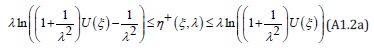
Similarly, by λ − invariance , the negative root satisfies
From Eqs. (A1.2) the lower and upper bounding of the roots η ± (ξ ,λ ) of Eq. (14) enables to prove Theorem 2. From Eq. (40), the period depends on the magnitude of the positive interval η + (ξ ,λ ) −η − (ξ ,λ ) . Upon introducing the “outer limit” Δout( ξ ,λ ) as
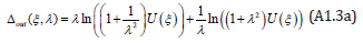
It is readily seen that Δout( ξ ,λ ) is a positive, increasing function of λ when λ ≥1 (and decreasing when λ ≤1) whose partial derivative ∂Δout( ξ ,λ ) /∂λ vanishes when λ =1. Similarly, upon introducing the “inner limit” Δin( ξ ,λ ) as
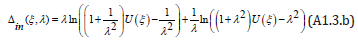
It is also seen that Δin( ξ ,λ ) is a positive, increasing function of λ when λ ≥1 (and decreasing when λ ≤1) whose partial derivative ∂Δin( ξ ,λ ) /∂λ also vanishes when λ =1. Since the positive interval η + (ξ ,λ ) −η − (ξ ,λ ) obviously satisfies

This proves Theorem 2.
Appendix 2
Upon recalling the definition (13) of U (ξ ), the solution (25a) is expressed as
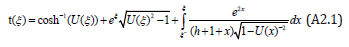
Since 1≤U (ξ ) ≤ eh , a binomial expansion of the integrand with binomial coefficients expressed in terms of the Gamma function Γ( p) yields an exact solution in terms of a converging series
The first integral ( p = 0) is directly expressed in terms of the exponential integral function Ei (x) , with the argument x > 0
When inserted into (A2.2) this expression provides a zeroth order ( p = 0) solution for t (ξ ) , hence for ξ (t ) = t−1 (ξ ) as discussed earlier.
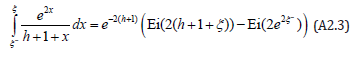
When the integer p is 1, 2, 3, . . . , each integral I2p(ξ) in (A2.2) is of the form

Successive integration by parts and substitution into (A2.2) result in a convergent series of exponential integral functions with positive argument of the form e−2 p(h+1)Ei(2 p (h + 1 +ξ )) .
Appendix 3
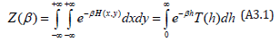
Based on thermodynamics, Rothe [22] established that the Laplace transform of the period functionT (h) , in which h is the system’s energy, is the canonical state sum Z (β ) of the Hamiltonian (6), with β ∈(0,∞) as the inverse of the absolute temperature, namely
From Eqs. (10) and (7) together with the definition (11) of the G-function, the LV system’s Hamiltonian is
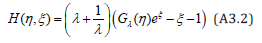
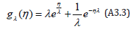
For notation purposes, we introduce the reduced g − function gλ (η) defined as
Consequently, upon inserting the Jacobian  of the linear
transformation (9)
of the linear
transformation (9)
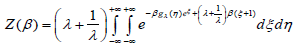
Upon substituting s = eξ with s ∈(0, ∞) , (A3.4) becomes
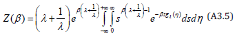
The integration over s is expressed in terms of the Gamma function Γ(s) :
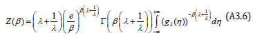
Together with the above definition of gλ (η) this definite integral has been evaluated (see 3.314 in [25]); the λ − invariant state sum Z (β ) thus becomes
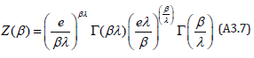
Although the Hamiltonian (A3.2) is defined in the ξ −η space, the result (A3.7) for the state sum Z (β ) is identical to that of Rothe (Eqs. (9) and (10) in [22]) who used the ”planar” Hamiltonian (6) in the x − y space. The derivation of the period then directly follows Rothe who defines a function τ (h) (Eqs. (15), (16), and (17) in [22]) whose Laplace transform is
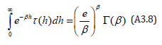
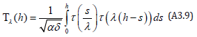
Since our state sum (A3.7) is expressed as the product of two Laplace transforms similar to (A3.8), use of the Hamiltonian (A3.2) establishes that the period Tλ (h) of the LV system (17) is directly equivalent to that of Rothe. Upon recalling the earlier definition of the dimensionless time, the period is expressed as a λ − invariant convolution integral satisfying Theorem 1 with τ (h) defined above
References
- Boulnois JL (2022) Predator-Prey linear coupling with hybrid species. arXiv 2301.00673.
- Boulnois JL (2023) An exact closed-form solution of the Lotka-Volterra equations. arXiv 2303.09317.
- Volterra V (1926) Variation and fluctuations of the number of individuals of animal species living together. In: Chapman RN (Ed.), Animal Ecology. McGraw-Hill, pp. 31-113.
- Lotka AJ (1920) Undamped oscillations derived from the law of mass action. J Am Chem Soc 42(8): 1595-1599.
- Doob JL (1936) Review: V Volterra Le¸cons sur la th´eorie math´ematique de la lutte pour la vie. Bull Amer Math Soc 42(5): 304-305.
- Chauvet E, Paullet JE, Previte JP, Walls Z (2002) A Lotka-Volterra three-species food chain. In Mathematics Magazine 75: 243-255.
- Chen-Charpentier BM, Stanescu D (2013) Virus propagation with randomness. Math and Comp Modelling 57(7-8): 1816-1821.
- Treanor CE, Rich JW, Rehm R (1968) Vibrational relaxation of anharmonic oscillators with exchange-dominated collisions. J Chem Phys 48:1798-1807.
- Frame J (1974) Explicit solutions in two species volterra systems. Journal of Theoretical Biology 43(1): 73-81.
- Evans CM, Findley GL (1999) A new transformation of the Lotka-Volterra problem. J Math Chem 25: 105-110.
- Mingari Scarpello G, Ritelli D (2003) A new method for the explicit integration of Lotka- Volterra equations 11(1): 1-17.
- Murty KN, Rao DVG (1987) Approximate analytical solutions of general Lotka-Volterra equations. J Math Anal Appl 122(2): 582-588.
- Rao DVG, Thorani YLP (2010) A study of the solutions of the Lotka-Volterra prey- predator system using perturbation technique. Int Math Forum 5(53-56): 2667-2673.
- Chowdhury MSH, Hashim I, Mawa S (2009) Solution of prey-predator problem by numeric- analytic technique. Commun Nonlinear Sci Numer Simul 14(4): 1008-1012.
- Shih SD (1997) The period of a Lotka-Volterra system. Taiwanese J Math 1(4): 451-470.
- Shih SD (2005) Comments on “A new method for the explicit integration of Lotka-Volterra equations”. Divulgaciones Matem´aticas 13(2): 99-106.
- Kerner EH (1964) Dynamical aspects of kinetics. Bull Math Biophys 26: 333-349.
- Kerner EH (1997) Comment on Hamiltonian structures for the n-dimensional Lotka-Volterra equations. J Math Phys 38(2): 1218-1223.
- Plank M (1995) Hamiltonian structures for the n-dimensional Lotka-Volterra equations. J Math Phys 36(7): 3520-3534.
- Waldvogel J (1986) The period in the Lotka-Volterra system is monotonic. J Math Anal Appl 114(1): 178-184.
- Hsu SB (1983) A remark on the period of the periodic solution in the Lotka-Volterra system. J Math Anal Appl 95(2): 428-436.
- Rothe F (1985) The periods of the Volterra-Lotka system. J Reine Angew Math 355: 129-138.
- Shih SD, Chow SS (2004) A power series in small energy for the period of the Lotka-Volterra system. Taiwanese J Math 8(4): 569-591.
- Grozdanovski T, Shepherd JJ (2007) Approximating the periodic solutions of the Lotka- Volterra system. ANZIAM J 49((C)): C243-C257.
- Gradshteyn IS, Ryzhik IM (1965) Table of integrals, series, and products. (4th edition). In: Geronimus JV and Ce˘ıtlin MJ (Eds.), Translated from the Russian by Scripta Technica Inc. Translation edited by Alan Jeffrey. Academic Press, New York-London, UK.
- Varma VS (1977) Exact solutions for a special prey-predator or competing species system. Bull Math Biology 39(5): 619-622.


 We use cookies to ensure you get the best experience on our website.