Research Article 
![]() Creative Commons, CC-BY
Creative Commons, CC-BY
Estimating Three Key Parameters from Measurements in Experiments of Heat Induced Flight
*Corresponding author: Hong Zhou, Department of Applied Mathematics, Naval Postgraduate School, Monterey, CA 93943, USA.
Received: June 08, 2023; Published: June 15, 2023
DOI: 10.34297/AJBSR.2023.19.002563
Abstract
We study the problem of heat-induced flight action when a subject is exposed to a millimeter wave beam. There are three key parameters in the model: the nociceptor activation temperature, the subjective threshold for flight initiation, and the human reaction time. We explore mathematical formulations for inferring the three parameters from data measured in exposure tests using the method of limit. We find that the simultaneous inference of the three parameters depends on the experimental design in the sequence of exposure tests. When the beam power density and beam radius of exposure tests span a rectangular region along its two diagonal directions, the three parameters are robustly estimated. Future experiments should consider this pattern of beam power density and beam radius when designing exposure tests. In the case of fluctuating subjective threshold, the medians of three parameters are still reliably estimated when the relative uncertainty in subjective threshold is small or moderate.
Keywords: Heat-induced flight, Activation temperature of thermal nociceptors, Subjective threshold for initiating flight, Human reaction time, Method of limits
Introduction
In cognitive neuroscience one of the main focuses is to understand the underlying mechanism that causes changes in behavior and neural responses through experimental investigation. There are two commonly adopted methods that can help us start psychophysical experiments: the method of limits [1-3] and the method of constant stimuli [1,3,4]. These two methods can be applied to study the response of a human subject exposed to a millimeter wave heating. During millimeter wave exposure, the electromagnetic energy is absorbed by the skin and thereby increases the skin temperature. Once the local temperature of the skin reaches the activation temperature, thermal nociceptors in the skin are activated to transduce an electrical signal. The strength of the total electrical signal is proportional to the number of activated nociceptors. When the pain signal transmitted from nociceptors to the brain is strong enough, the brain issues an instruction signal, directing the muscles to execute a flight action. A flight action here refers to escaping from the electromagnetic beam and/or switching off the beam power. When a test subject is exposed to a time invariant millimeter wave beam, the total amount of activated nociceptors and the electrical signal transduced by the activated nociceptors both rise with the exposure duration. There is a subjective threshold on the exposure duration for the pain signal to reach the subjective tolerance for inducing the flight action. Due to the bio-variability (both the lateral and longitudinal), this subjective threshold is a random variable, fluctuating from one subject to another and fluctuating from one test to another on the same subject. We view the flight action as initiated when the electrical signal transduced at the exposed skin spot by thermal nociceptors is sufficient for triggering the flight instruction upon propagating to the brain. It takes time for the pain signal to travel from the exposed skin spot to the brain, for the brain to process the pain signal and to issue a flight instruction, and for the muscles to receive the flight instruction and carry out the flight action. As a result, the time of observed flight action is delayed from the time-of-flight initiation. This time delay is the human reaction time.
In our recent work [5] we extracted the median subjective threshold on exposure duration and the human reaction time from data measured in exposure tests designed using the Method of Constant Stimuli (MoCS) where the exposure duration is prescribed in each test. The data collected in a sequence of tests include prescribed exposure durations, observed binary outcomes regarding the occurrence of flight action, and times of observed flight action (if flight occurs). In each test of MoCS, flight action may or may not occur depending on whether the prescribed exposure duration is above or below the sample subjective threshold in that test. In a sequence of exposure tests, the prescription of exposure duration for the next test is updated adaptively based on the prescriptions and outcomes in the tests already completed, using a Bayesian framework. The goal is to probe the system near the median subjective threshold where the human response is most uncertain (about 50% each way). We modeled the random subjective threshold as a Weibull distribution and carried out the inference in two steps. In step 1, we infer the median subjective threshold from the observed binary outcomes, which are independent of the human reaction time. In step 2, we combine the result from step 1 and the times of observed flight action in an inference framework to estimate the deterministic human reaction time. The inference method developed is robust with respect to the discrepancy between the inference model assumed and the actual model of the data. Although the inference method is formulated assuming the Weibull distribution, it yields correct results on the data generated using other distributions for the random subjective threshold. In this paper, we work with data measured in exposure tests designed using the Method of Limits (MoL) where the beam power is kept on and steady until the flight action is observed in each test. The data set contains a sequence of data elements, each corresponding to an individual test. Each data element consists of beam specifications used (beam radius and beam power density), the time series of measured skin surface temperatures (recorded by an IR camera), and the time of observed flight action in an individual test. Previously, we developed a method for reconstructing the skin internal temperature distribution from a time series of surface temperatures [6]. The reconstruction of internal temperature distribution is parameter free. Thus, although the internal temperature distribution is not directly measured in exposure tests, we can regard it as part of the data for inference.
The data of reconstructed skin internal temperatures allow us to examine the process of nociceptor activation and the flight initiation. In this process, there are three key parameters: the activation temperature of thermal nociceptors, the subjective threshold on activated volume for initiating flight and the human reaction time. In this study, we explore the inference of these three key parameters from data in tests of MoL. In each test of MoL, upon the start of beam power, the skin temperature increases monotonically. Thermal nociceptors are activated when the local temperature reaches the activation temperature (which we regard as unknown). Under the assumption that nociceptors are uniformly distributed in skin, the total electrical signal transduced by the nociceptors is proportional to the activated volume where the temperature is above the activation temperature. We use the activated volume to measure the pain signal. There is a subjective threshold on the activated volume.
When this threshold is exceeded, the total electrical signal transduced is sufficient for inducing flight action. We regard this time instance as the flight initiation time. The time of observed flight action is delayed from the flight initiation time by the human reaction time. In a test of MoL, flight action always occurs. The time of observed flight action is influenced by 0) the skin internal temperature distribution, i) the nociceptor activation temperature, ii) the subjective threshold on activated volume for initiating flight, iii) the human reaction time. Item 0) is part of the data we work with; items i)-iii) are the target of our inference analysis. In this study, we focus on the case where both the nociceptor activation temperature and the human reaction are deterministic while the subject threshold on activated volume is allowed to be a random variable, for which we aim at estimating the median. The objective of this study is to develop a mathematical framework for extracting the three key parameters i)-iii) listed above, from data of beam specifications, skin internal temperature distributions, and times of observed flight action measured in tests of MoL. The mathematical framework includes both the inference component and the experimental design component for optimizing the inference. We explore the advantage of having a set of exposure tests spanning a significant range both in the beam radius and in the beam power density used in tests.
Model Of Flight Action in The Method of Limits
Coordinate System and Temperature Distribution
We establish the coordinate system as follows. The skin surface exposed to the millimeter wave is selected as the xy plane with the 2D coordinates denoted by vector r = (x, y); the depth into the skin is selected as the z-direction. A point in the skin tissue is completely described by its 3D coordinates (r, z). Let T(r, z, t) be the skin temperature at position (r, z) at time t, which increases monotonically with t upon the start of beam power. We use the notation {T(r, z, t)} to represent the skin internal temperature distribution. In exposure experiments, the skin surface temperature distribution, {T(r, z = 0, t)}, is recorded with an IR camera at a sequence of discrete time instances. In a previous study [6], we developed a method for reconstructing the skin internal temperature distribution from a time series of measured skin surface temperatures. The reconstruction method is based solely on the measured surface temperatures; it does not require any parameter values of skin material properties. The reconstruction of skin internal temperature distribution is carried out individually for each exposure test. For this reason, we treat the skin internal temperature distribution as measurable even though it is not directly measured in exposure tests.
Flight Initiation and Flight Actuation as Determined by the Skin Temperature Distribution
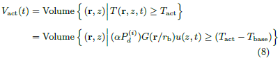
Upon the start of beam power, the absorbed electromagnetic energy increases the skin temperature, activates the thermal nociceptors, and produces a heat sensation on the exposed subject. Eventually, when the heat sensation exceeds a threshold, the exposed subject escapes from the beam (we shall call this the flight action) [7,8]. Let Tact be the activation temperature of thermal nociceptors. We adopt the model used in [9] that the initiation of flight is governed by the number of activated nociceptors relative to a subjective threshold. Under the assumption that the thermal nociceptors are uniformly distributed in skin tissue, the number of activated nociceptors at time t is directly proportional to the activated volume Vact(t), the volume of the 3D region in which the skin temperature at time t is above the activation temperature.

Given the temperature distribution {T(r, z, t)}, the activated volume {Vact(t)} is determined by the activation temperature Tact. In exposure tests using the method of limits, the beam power is kept on and steady. The skin temperature and the activated volume increase monotonically with t until the beam power is turned off at the time of flight actuation.
The time of flight initiation is governed by {Vact(t)} relative to a subjective threshold vc on Vact. Let tc be the time at which the activated volume reaches the subjective threshold vc.
At time tc, the electrical signal transduced by thermal nociceptors at the exposed skin spot is strong enough such that after propagating to the brain, it triggers the brain to issue a flight instruction signal to muscles, which eventually actuates the flight action. The process of flight actuation beyond time tc is irreversible. Even if the beam power is turned off right at tc, the electrical signal already generated by time tc will still lead to flight action. Thus, we view tc as the time of flight initiation. Mathematically, the flight initiation time tc is governed by
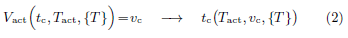
Given the temperature distribution {T(r, z, t)}, the flight initiation time tc is determined by the activation temperature Tact and the subjective volume threshold vc.
The flight action occurs at time tF, later than the flight initiation time tc. The time delay, tR ≡ tF − tc, is the human reaction time. We summarize the quantities and functions introduced above.
• r = (x, y): lateral coordinates on the skin surface.
• z: depth into the skin tissue; (r, z) is the 3D coordinates of a point in the skin.
• t: time (t = 0 is set as the time when the beam power is turned on).
• T(r, z, t): skin temperature at position (r, z) at time t.
• {T} ≡ {T(r, z, t)}: skin internal temperature distribution.
• Tact: activation temperature of thermal nociceptors.
• Vact(t) ≡ Vact(t, Tact, {T}): activated volume of skin tissue at time t.
• vc: subjective threshold on activated volume for initiating flight.
• tc: flight initiation time governed by Vact(t, Tact, {T})=vc; given temperature distribution {T}, tc is influenced by parameters Tact and vc.
• tR: human reaction time.
• tF = tc + tR: time of observed flight action; given temperature distribution {T}, tF is influenced by Tact, vc and tR, the three model parameters we want to infer.
Data from exposure tests and inference objectives
In each exposure test, the time of observed flight action tF is recorded while the skin internal temperature distribution T(r, z, t) is indirectly measured, i.e., constructed from a time series of skin surface temperature distributions recorded with an IR camera.
None of Tact, vc, tR, Vact(t) or tc is directly measurable. We explore the possibility of inferring from measured data the three key parameters: Tact, vc and tR. In this study, we allow vc, the subjective volume threshold, to be a random variable, fluctuating from one subject to another and fluctuating from one test to another on the same subject; we assume Tact and tR are deterministic unknowns. Our goal is to infer Tact, median(vc) and tR from data (Figure 1).
In exposure tests using the method of limits, the data set measured in a sequence of N tests, after post processing, has the form

where  is the beam center power density of the incident
beam used in test j, and (AHM)j is the half-maximum area
of the beam cross-section. Figure 1 illustrates the process from
the start of beam power to the observed flight action in an exposure
test, based on the model described above. In the process,
none of (Tact, Vact(t), vc, tc, tR) is measurable in real experiments.
Only tF and {T(r, z, t)} are measurable and included in
data format (3). As we will see, the values of ( , (AHM)j) are not directly used in the inference of (Tact, vc, tR). However,
a robust inference depends on data from a diversified sequence
of exposure tests that spans a significant range in the 2D domain
of {}, {(AHM)j}. In particular, if all exposure
tests in the sequence use the same beam power density and the
same beam spot area, it is impossible to infer more than one
parameter.
is the beam center power density of the incident
beam used in test j, and (AHM)j is the half-maximum area
of the beam cross-section. Figure 1 illustrates the process from
the start of beam power to the observed flight action in an exposure
test, based on the model described above. In the process,
none of (Tact, Vact(t), vc, tc, tR) is measurable in real experiments.
Only tF and {T(r, z, t)} are measurable and included in
data format (3). As we will see, the values of ( , (AHM)j) are not directly used in the inference of (Tact, vc, tR). However,
a robust inference depends on data from a diversified sequence
of exposure tests that spans a significant range in the 2D domain
of {}, {(AHM)j}. In particular, if all exposure
tests in the sequence use the same beam power density and the
same beam spot area, it is impossible to infer more than one
parameter.

Figure 1: An exposure test using the method of limits. Measurable and non-measurable quantities in the experimental process of inducing flight action.
Model of Experimental Data on Skin Temperature Distribution and Data Generation
Skin Temperature Evolution When Exposed to a Beam
We consider the situation where the skin area of a test subject is exposed to a beam of millimeter wave [10-12]. We adopt a model of skin temperature evolution like that in our previous studies [13-15]. The model is based on the assumptions below.
1. The skin surface exposed to the millimeter wave is flat (the xy plane).
2. The beam ray is along the z-direction, perpendicular to the skin surface.
3. In the xy plane, the beam power density has an axisymmetric Gaussian distribution.
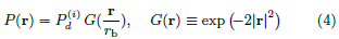
where rb is the Gaussian beam radius [16]. Here the assumption of axisymmetry is only for simplicity in analysis. The scaling relation between the beam spot area and the activated volume remains the same for all types of beam power distributions.
4. The skin’s material properties are uniform in (z, r).
5. The length scale in the lateral directions rb is much larger than the penetration depth of millimeter wave into the skin (less than 0.5 mm) [17]. In the leading order approximation, the temperature evolution is dominated by the the conduction along the z-direction and the effect of lateral heat conduction is neglected.
6. In exposure tests, the beam power density is selected high enough to ensure that flight action occurs in a short time [7,8]. During this short time period, the cooling effects of blood circulation and heat loss at the skin surface are neglected.
7. Before the start of beam power, the skin’s initial temperature is uniform in (z, r), which is called the skin baseline temperature and is denoted by Tbase.
Let t = 0 be the beam start time. The temperature distribution T(r, z, t) is governed by
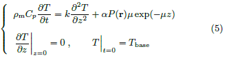
Where,
• ρm is the mass density of the skin,
• Cp is the specific heat capacity of the skin,
• k is the heat conductivity of the skin,
• μ is the absorption coefficient of the skin for the beam frequency used,
• P(r) is the Gaussian distribution of beam power density in (4), and
• α is the fraction of incident beam power absorbed into the skin.
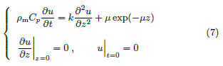
Since the lateral heat conduction is neglected, (5) does not
involve any derivative with respect to lateral coordinate r. The
dependence on r is only in the heat source term via P(r) ≡
 G(r/rb). This allows us to write the solution of (5) as

where u(z, t) is the temperature increase per unit of absorbed beam power density and is governed by
The activated volume at time t is
Nondimensionalization
The activated volume given in (8) is affected by many parameters:
• the absorbed beam power density (α),
• rb in Gaussian distribution G(r/rb),
• (ρm, Cp, k, μ) in the temperature increase per unit of absorbed beam power density u(z, t),
• (Tbase −Tact) on the right hand side of the inequality. The initiation of flight is determined by the activated volume relative to the subjective threshold vc. In total, there are 9 physical quantities affecting the initiation of flight, namely.

To reveal the roles and interactions of these physical quantities in initiating flight action, and to simplify the mathematical formulation, we carry out non-dimensionalization. For each physical quantity, we introduce a scale for its physical dimension and write out the corresponding non-dimensional quantity.
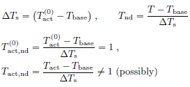
• Temperature scale is the difference between a characteristic
activation temperature  and the baseline temperature
Tbase. The true Tact may deviate from
and the baseline temperature
Tbase. The true Tact may deviate from
• Length scale in the depth direction is provided by, 1/μ, the characteristic penetration depth of millimeter wave into the skin.

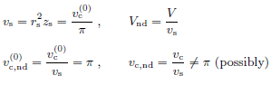
• Length scale in the lateral directions is obtained from a
characteristic volume threshold  . The true volume
threshold vc may deviate from .
. The true volume
threshold vc may deviate from .

Geometrically, rs is the radius of the cylinder with volume and height zs.
• Volume scale is provided by the combination r2 s zs.
• Time scale is derived from skin material properties.
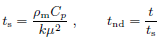
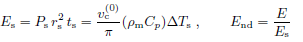
• Power density scale is derived from vs, (ρmCp), ΔTs, rs, and ts.

• Scale for u ≡ (T − Tbase)/(αP), temperature per power density, is

• Energy scale is built based on Ps, ts, and rs.
We need to point out that in the non-dimensionalization
above, we used a characteristic activation temperature and
a characteristic volume threshold . The actual values of
(Tact, vc) may deviate from (, )
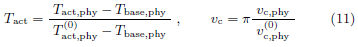
For simplicity, we shall drop the subscript nd in all nondimensional
quantities. Instead, the original physical quantities
will be distinguished with subscript phy, when necessary
for clarity. For example, refers to the non-dimensional
beam center power density while  is the physical beam
center power density before non-dimensionalization. With this
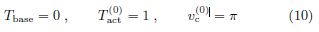
notation, the non-dimensional versions of baseline temperature,
characteristic activation temperature and characteristic volume
threshold are
is the physical beam
center power density before non-dimensionalization. With this
notation, the non-dimensional versions of baseline temperature,
characteristic activation temperature and characteristic volume
threshold are
The non-dimensional version of true (Tact, vc) may deviate
from (, ).
After nondimensionalization, (7), the evolution equation of the temperature increase per beam power density u(z, t) becomes
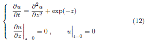
Equation (12) is parameter free. Its solution has a closedform expression [18].
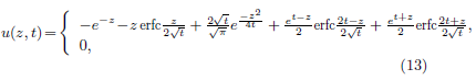
where erfc(u) is the complementary error function defined as

The absorption fraction α and the beam center power density
appear only in the combination (α ). For conciseness,
we rename the combination as Pd ≡ (α ). It follows
from (6) that the non-dimensional temperature distribution is
completely described by parameters (Pd, rb) and has the expression.

where the non-dimensional version of (Pd, rb) is

The corresponding non-dimensional activated volume at time t is

A change of variables rnew = rold/rb separates out the dependence on rb.

Scaling relation (18) greatly simplifies the calculation of Vact(t) for various values of (Tact, Pd, rb).
The temperature per unit power density u(z, t) in (13) increases monotonically with t.

It follows that the activated volume Vact(t) increases monotonically with t. Flight is irreversibly initiated at tc when Vact(t) reaches the subjective threshold vc. The flight initiation time tc is related to parameters (Tact, vc, Pd, rb) in the equation below

Upon being initiated at time tc, flight is eventually materialized and observed at time tF = tc + tR > tc where tR is the human reaction time.
In summary, from the start of beam power to the time of observed flight action, the non-dimensional process has only 5 parameters: (Tact, vc, tR, Pd, rb), in which (Pd, rb) are the beam specifications that we select in experimental design; (Tact, vc, tR) are the unknown parameters we try to infer from data of (tF, {T}).
Model of the randomness in subjective threshold vc
Of the three key model parameters (Tact, vc, tR), in this study,
we assume the activation temperature Tact and the human reaction
time tR are deterministic while allowing the subjective
threshold vc to be a random variable. The objective of our inference
is to estimate the deterministic quantities (Tact,  , tR) where ≡ median(vc). In our numerical simulations, we test
inference performance on data sets generated respectively from
a Weibull distribution or from a log-normal distribution for vc.
, tR) where ≡ median(vc). In our numerical simulations, we test
inference performance on data sets generated respectively from
a Weibull distribution or from a log-normal distribution for vc.
• Weibull distribution for vc
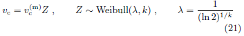
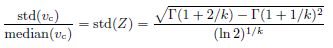
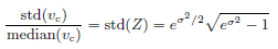
The scale parameter λ is related to the shape parameter k as given above to make median(Z) = 1. Random variable Z has only one parameter k, which governs the distribution width. The relative standard deviation of vc is
• Log-normal distribution for vc
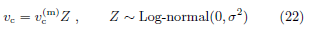
Random variable Z satisfies median(Z) = 1 and has only one parameter σ, which governs the distribution width. The relative standard deviation of vc is
Generating Artificial Data Based on the Model
The non-dimensionalization in the previous subsection is based
on ( , ), a characteristic activation temperature and a
characteristic volume threshold. This approach simplifies the
formulation and at the same time allows us to consider the true
activation temperature and the true volume threshold (Tact, vc)
as unknown parameters in the system. We will generate data
and carry out inference analysis in this non-dimensional system.
At the end, we will show that the inference methods developed
are invariant under scaling. Thus, the inference methods developed
are directly applicable to real experimental data.
We generate artificial data sets of the format described in
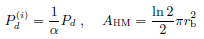
(3). The incident beam power density is directly proportional
to the absorbed beam power density Pd. The half maximum
area of beam spot AHM is proportional to  , the square
of beam radius.
, the square
of beam radius.
For simplicity we adopt the format in (23) for artificial data sets.
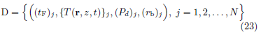
This change in data format does not affect the inference. We use the values of {(Pd)j , (rb)j} only to indicate the diversity of exposure tests in beam power density and in beam spot size.
The values of {(Pd)j , (rb)j} do not actually enter into the inference computation.
We use the parameters below in our data generation.
An artificial data set consists of data elements from a sequence of exposure tests, each data element containing the results of an individual test. These tests are divided into groups accordingly to their values of (Pd, rb). We follow the steps below to generate the data element for each individual test.
i) For each test, select (Pd, rb) according to the experimental design.
ii) With (Pd, rb), build the temperature distribution {T(r, z, t)} in (15), which corresponds to the skin internal temperature distribution reconstructed from the time series of skin surface temperatures measured in a real test.
iii) With {T(r, z, t)} and Tact, calculate the activated volume {Vact(t)} in (18).
iv) Draw a random sample of vc according to distribution (21,22).
v) With {Vact(t)} and vc, solve for the flight initiation time tc in (20).
vi) With tc and tR, calculate the flight actuation time tF = tc + tR.
vii) The data element for the test is (tF, {T(r, z, t)}, Pd, rb).
For each test in the data generation, a sample of vc is drawn from distribution (21,22). The sample is used to calculate tc, which leads to tF. While tF is recorded in data, neither vc nor tc is included in data because neither is measurable in experiments. To emulate the situation of real exposure tests, the artificial data include only the measurable quantities.
Mathematical Formulation and Experimental Design for Inference
We explore mathematical formulations for inferring
(Tact, vc, tR) from a given data set. Since not all data sets
contain the necessary information for determining (Tact, vc, tR),
we also examine the experimental design behind the data collection/
generation to optimize the inference performance. In
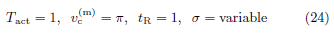
this section, for simplicity, we work with data sets generated
using deterministic vc (i.e., vc = in (21) and (22)).
Our general strategy is to analyze the ensemble behavior of the activated volume. In each individual tests, we calculate the activated volume using trial parameter values. Then we study the ensemble behavior of activated volume over all exposure tests. This ensemble behavior is the key in revealing information about our inference target (Tact, vc, tR), and is highly influenced by the diversity of the exposure tests in (Pd, rb). Specifically, we focus on the predicted activated volume at the predicted time of flight initiation because this quantity is invariant over all exposure tests when the trial parameter values used in predicting the activated volume coincide with the true parameter values.
Given the skin temperature distribution in data, the activated volume as a function of t is readily calculated when a trial value of the activation temperature Tact is supplied (Figure 2). The time of flight initiation is predicted from the time of observed flight action in data and a trial value of the human reaction time tR (Figure 2). Combining the two steps, we predict the activated volume at flight initiation for each pair of trial values of (Tact, tR).
In each individual exposure test, the predicted activated
volume at flight initiation is a function of ( ,
,  ). From
a data set containing a sequence of tests, we obtain a collection
of such functions, one for each test.
). From
a data set containing a sequence of tests, we obtain a collection
of such functions, one for each test.
Activated volume at flight initiation Vc calculated from data using trial values of (Tact, tR)
Let Vc denote the activated volume at the time of flight initiation,
Given the skin temperature distribution in data (23), the calculation of Vc in (25) depends on the activation temperature Tact and the time of flight initiation tc = tF − tR where tF is the time of observed flight action given in data. Thus, given the data of an individual test, the calculation of Vc in (25) is completely specified by the trial values of (Tact, tR). Figure 2 illustrates the 3 steps in calculating Vc from data.
i) Given a trial value of activation temperature ,
the temperature distribution {T(r, z, t)} in data produces
{Vact(t; )}.
ii) Given a trial value of the human reaction time , the
time of observed flight actuation tF in data gives tc = tF −
.
iii) Combining {Vact(t)} and tc, we obtain Vc( , ) ≡ Vact(tc; ).
For conciseness, we drop the superscript (trial) and denote
the trial values simply by (Tact, tR). Data set (23) contains
a sequence of N exposure tests. From the data of test j, we
calculate the two-variable function Vc,j(Tact, tR), the activated
volume at flight initiation predicted using trial values (Tact, tR).
The calculated function Vc,j(Tact, tR) is specific to test j and is
affected by the beam parameters (rb, Pd) used in test j. For
data set (23), we have a family of N calculated Vc,j(Tact, tR).

Note that the true volume threshold vc is the true activated volume at the true time of flight initiation, all of which are unknown. The calculation of Vc,j(Tact, tR) does not require vc. The unknown vc and the family of calculated functions (26) are related by

Figure 2: The activated volume at flight initiation, calculated from data ({T(r, z, t)}, tF), as a function of trial parameters
( , ).
At each point in the 2D space of (Tact, tR), (26) gives a set of N calculated values of Vc,j . We study the normalized sample standard deviation of the set, SV , defined below.

where δ is a tiny number much smaller than the true volume
threshold vc (e.g., δ = 10−40). At true values ( ,
,  ),
(27) gives
),
(27) gives

Since SV (Tact, tR) ≥ 0 everywhere, we estimate
( , ) by minimizing SV .
Once ( ,
,  ) is obtained, we estimate ≡ median(vc) as
(Eq 28), (Eq 30) and (Eq 31) provide the mathematical
foundation for inferring ( , , ).
The definition of SV in (28) is selected for two purposes:
1. we normalize the std to measure the relative changes in Vc instead of the absolute changes;
2. we use a tiny number δ to mitigate the singularity when mean{Vc,j} = 0.
This singularity occurs when the trial value of Tact is too
high. At a high activation temperature, no nociceptor is
activated and the predicted activated volume is zero for all
tests in the data set. As a result, we have mean{Vc,j} = 0,
std{Vc,j} = 0 and d = δ for large Tact. To make the minimum
in (30) uniquely and robustly defined at the true target
( , ), we use a tiny number δ to make SV (Tact, tR)
large for large Tact.
Calculated SV (Tact, tR) on a data set spanning a range of power density at a fixed beam radius
As described in equation (30), our approach of estimating
( , ) is to minimize the two-variable function
SV (Tact, tR), which is calculated from data. The success of
this approach depends on that SV (Tact, tR) has a uniquely defined
minimum. In particular, we need SV (Tact, tR) > 0 away
from ( , ). This requires that the exposure tests in
the data set span a significant range in the beam power density
Pd direction and/or in the beam radius rb direction. In
the absence of noise/uncertainty, if all tests in a data set have
the same (Pd, rb), then all tests will produce the same temperature
distribution of {T} and the same value of tF, which
yields the same calculated value of Vc,j(Tact, tR) for all j. It
leads to std{Vc} = 0 everywhere and SV (Tact, tR) = 0 in the
parameter region where mean{Vc} > δ, which is a large region
in (Tact, tR). To make SV = 0 only at ( , ), the
exposure tests need to have a significant diversity in (Pd, rb).
In this subsection, we study SV (Tact, tR) on a data set spanning a range of Pd at a fixed rb. Figure 3 shows the (rb, Pd)- distribution of the data set (left panel) and the contour plot of SV (Tact, tR) calculated from the data set (right panel). From the contour plot, we see that the minimum of SV (Tact, tR) in the 2D space of (Tact, tR) is practically attained everywhere in a slender ellipse, which is approximately aligned with the Tact direction. The 2D minimum is not robustly defined. We study the problem of determining one of (Tact, tR) while the other is known. When tR = 1 is given, the plot of SV vs Tact is fairly flat (left panel of Figure 4). In contrast, when Tact = 1 is given, the plot of SV vs tR has a well-defined minimum (right panel of Figure 4).
Conclusions of Figures 3 and 4
We examine the inference of (Tact, tR) from a data set of exposure tests spanning a range of power density at a fixed beam radius. This data set is ineffective for inferring (Tact, tR) simultaneously. The 2D inference is susceptible to noise and errors. The activation temperature Tact is not robustly determined even if the true human reaction time tR = 1 is given. On the other hand, if the true activation temperature Tact = 1 is given, the human reaction time tR is very well-determined.

Figure 3: Left: (rb, Pd)-distribution of the data set spanning a range of Pd at a fixed rb. Right: contours of SV vs (Tact, tR) based on the data set.

Figure 4: Left: SV vs Tact at tR = 1 based on the same data as in Figure 1. Right: SV vs tR at Tact = 1.
Calculated SV (Tact, tR) on a data set spanning a range of beam radius at a fixed power density
In this subsection, we study SV (Tact, tR) on a data set spanning a range of rb at a fixed Pd. Figure 5 shows the (rb, Pd)- distribution of the data set (left panel) and the contour plot of SV (Tact, tR) calculated from the data set (right panel). From the contour plot, we see that the minimum of SV in the 2D space of (Tact, tR) is not well-defined at all. The minimum is virtually attained everywhere in a straight deep valley along the angular direction of 3π/4. We study the problem of determining one of (Tact, tR) while the other is known. When tR = 1 is given, the plot of SV vs Tact has a well-defined minimum (left panel of Figure 6). Similarly, when Tact = 1 is given, the plot of SV vs tR also demonstrates a well-defined minimum (right panel of Figure 6).
Conclusions of Figures 5 and 6. We examine the inference of (Tact, tR) from a data set of exposure tests spanning a range of beam radius at a fixed power density. This data set does not contain enough information for inferring (Tact, tR) simultaneously. Only the combination (Tact + tR) is accurately extracted from the data while (Tact − tR) is virtually undetermined. However, if one of (Tact, tR) is given, the other is very well-determined.
Calculated SV (Tact, tR) on data sets with more widespread (rb, Pd)-distributions
To infer (Tact, tR) simultaneously, we need data sets of exposure
tests with more diversity in (rb, Pd). We examine the inference
performance of 3 different data sets, each covering the 2D region
of (rb, Pd) in some way. In Figure 7, we consider the data set of
7 pairs of beam parameters covering both the beam radius and
the power density directions but not the 4 corners of the 2D
region (left panel). Due to its diversity in both rb and Pd, this
data set produces a well-defined minimum of SV in the 2D space
of (Tact, tR) (right panel). In Figure 8, we examine the full data
set containing all 16 pairs of beam parameters in the entire 2D
region of (rb, Pd) (left panel). Not surprisingly, the minimum of
SV in the 2D space of (Tact, tR) is much better defined based on
this data set (right panel). When (Tact, tR) moves away from
( , ), the value of SV increases much more rapidly in
Figure 8 than in Figure 7, which makes the inference more robust
with respect to noise and errors. Next we explore achieving
the inference robustness of Figure 8 with fewer than 16 pairs of
beam parameters. In Figure 9, the experimental design uses 8
pairs of beam parameters to cover the two diagonals of the 2D
region, which include the 4 corners (left panel). Because of this
excellent diversity in (rb, Pd), the data set in Figure 9 leads to
both an excellent robustness and a good efficiency in inferring
(Tact, tR) (right panel).
Conclusions of Figures 7,8 and 9
We examine the simultaneous inference of (Tact, tR) from a data set of exposure tests covering the 2D region of beam radius and power density. The 2D inference is well-defined and robust as long as the data set covers the 2D region in a genuine way. The most effective data set for inference consists of exposure tests with the (rb, Pd)-distribution covering the two diagonals of the 2D region, as illustrated in the left panel of Figure 9. We shall use this (rb, Pd)-distribution in our numerical tests with noise.

Figure 5: Left: (rb, Pd)-distribution of the data set spanning a range of rb at a fixed Pd. Right: contours of SV vs (Tact, tR) based on the data set.

Figure 6: Left: SV vs Tact at tR = 1 based on the same data as in Figure 3. Right: SV vs tR at Tact = 1.

Figure 7: Left: (rb, Pd)-distribution of the data set from 7 pairs of beam parameters covering the horizontal and vertical directions of the 2D region. Right: contours of SV vs (Tact, tR) based on the data set.
Inference performance on data with fluctuating vc
In this section, we test the performance of the inference method developed in Section 4 on data generated with fluctuating vc, the subjective threshold on activated volume. The randomness of vc is modeled as distribution (21) or (22).
Summary of the Inference Method and Experimental Design
Our inference approach formulated in Section 4 consists of the steps below.
i) In a data set of form (23), for test j, we calculate the activated volume at flight initiation Vc,j, using trial values of (Tact, tR), as described in Figure 2.
ii) The calculated Vc,j is a function of (Tact, tR). At each point in the 2D space of (Tact, tR), data set (23) yields a set of N calculated values of Vc,j . As defined in (28), the normalized sample standard deviation of the set is a function of (Tact, tR).

iii) As described in (30), we infer ( , ) by minimizing SV.


Figure 8: Left: (rb, Pd)-distribution of the data set from all 16 pairs of beam parameters in the 2D region. Right: contours of SV vs (Tact, tR) based on the data set.

Figure 9: Left: (rb, Pd)-distribution of the data set from 8 pairs of beam parameters covering the two diagonal directions of the 2D region. Right: contours of SV vs (Tact, tR) based on the data set.
iv) As given in (31), ≡ median(vc) is estimated from
Vc,j( , ).

v) In the presence of noise, the success of inference requires that SV have a robustly defined minimum in the 2D space of (Tact, tR), which depends on the diversity in beam parameters (rb, Pd) used in exposure tests. The most effective data set has the (rb, Pd)-distribution shown in Figure 9. We shall use this (rb, Pd)-distribution when generating artificial data sets in our numerical tests.
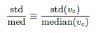
Inference results on data from the Weibull distribution
In this subsection, we test the performance of the inference method on data generated with random subjective threshold vc of the Weibull distribution. Histograms of vc are displayed in Figure 10 for std/med = 0.1, 0.2, 0.4 and 0.8 where “med” denotes “median”(Figure 10).
Note that with std/med = 0.4, the relative uncertainty is already unusually large for the subjective threshold. With std/med = 0.8, the relative uncertainty in vc is unrealistic. We include these large values of std/med in our numerical tests to demonstrate the trends of inference errors vs underlying uncertainty in vc.
In data generation, we use the (rb, Pd)-distribution in Figure 9, which consists of 8 pairs of (rb, Pd). At each pair of (rb, Pd), we run m independent exposure tests to sample the randomness of vc. The resulting data set contains N = 8m exposure tests. In numerical simulations below, N = 200 (m = 25) unless indicated otherwise.
In Figure 11, we plot contours of SV vs (Tact, tR) for
std/med = 0.1, 0.2, 0.4 and 0.8. In each panel, the minimum
of SV in the 2D space of (Tact, tR), shown as a red dot, gives
the inference results ( , ). It is clear that a larger uncertainty
in vc makes the surface of SV flatter, which in turn
makes the minimum more susceptible to perturbations.
Following the intuition gained in Figure 11, we use Monte
Carlo simulations to investigate the effects of std/med of vc
on the inference results.At every set of parameters, we repeat
the process of data generation and inference for M = 500
Monte Carlo runs, each yielding one set of estimated parameters
( , ,  ). From M = 500 Monte Carlo runs,
values of ( , , ) vs std/med of vc are presented
as scatter plots with associated box plots in 3 panels of Figure
12. These 3 quantities are inferred from data set (23), which
does not contain values of since it is not measurable in real experiments.
Of these 3 quantities, has the smallest relative
error; has the largest relative error. For comparison, we
also plot sample median of vc vs std/med of vc in the bottom
right panel of Figure 12. The sample median is calculated in the data generation process (23).
). From M = 500 Monte Carlo runs,
values of ( , , ) vs std/med of vc are presented
as scatter plots with associated box plots in 3 panels of Figure
12. These 3 quantities are inferred from data set (23), which
does not contain values of since it is not measurable in real experiments.
Of these 3 quantities, has the smallest relative
error; has the largest relative error. For comparison, we
also plot sample median of vc vs std/med of vc in the bottom
right panel of Figure 12. The sample median is calculated in the data generation process (23).

Figure 10: Histograms of vc for std/med = 0.1, 0.2, 0.4 and 0.8. The orange bar represents the bin of [9,+∞).

Figure 11: Contours of SV vs (Tact, tR) based on data with the std/med given.

Note that sample values of vc are not measurable in experiments.
As a result, the sample median cannot be calculated
from data set (23), which makes the sample median irrelevant
in real applications. Here we plot the sample median to demonstrate
an upper limit on the inference performance of
Even if we are given sample values of vc in the data set, statistically
we cannot estimate more accurately than the sample
median.
In each of the 3 panels for (, , ) in Figure
12, values of the estimated quantity show both a spreading
(the IQR box in box plots) and a systematic bias (the median
line in box plots). We examined the effects of sample size N on the spreading and the bias. Figure 13 compares values of
(, ) for N = 200 (top row) and for N = 800 (bottom
row); Figure 14 compares values of (,  ) for N =
200 (top row) and for N = 800 (bottom row), where N is the
number of exposure tests in a data set. In each panel, the two
dotted blue lines indicate respectively the 25th and the 75th
percentiles corresponding to the IQR box in box plots of Figure
12; the dotted red line indicates the median. Figures 13 and 14
demonstrate that as sample size N increases, the interquartile
range (IQR) of the inferred quantity decreases, proportional to
N−1/2. In contrast, the bias in the inferred quantity remains
unchanged as sample size N is increased.
) for N =
200 (top row) and for N = 800 (bottom row), where N is the
number of exposure tests in a data set. In each panel, the two
dotted blue lines indicate respectively the 25th and the 75th
percentiles corresponding to the IQR box in box plots of Figure
12; the dotted red line indicates the median. Figures 13 and 14
demonstrate that as sample size N increases, the interquartile
range (IQR) of the inferred quantity decreases, proportional to
N−1/2. In contrast, the bias in the inferred quantity remains
unchanged as sample size N is increased.

Figure 12: Top left: values of inferred from data vs std/med of vc. Top right: vs std/med. Bottom left: vs
std/med. Bottom right: sample median of vc vs std/med.

Figure 13: Histograms of (left) and (right) from Monte Carlo simulations with sample size N = 200 (top) and N = 800
(bottom).
Next we study the effects of std/med (relative uncertainty
in subjective threshold vc) on the relative spreading and the relative bias of an inferred quantity. We introduce two measures
of relative error in a quantity Q, which can be any of
(, , ).

Figure 14: Left: histograms of from Monte Carlo simulations with sample size N = 200 (top) and N = 800 (bottom).
Right: histograms of are plotted for reference only. is not available from experimental data.
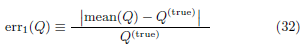
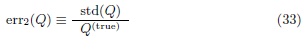
err1(Q) measures the relative bias in quantity Q while
err2(Q) measures the relative spreading in quantity Q. In Figure
15, for the 3 inferred quantities (, , ), we
plot err1 (left column) and err2 (right column) vs std/med of vc
as linear plots (top row) and as log-log plots (bottom row). The
straight line fittings in log-log plots demonstrate that for each
of the 3 inferred quantities, err1 is proportional to (std/med)2
while err2 is proportional to std/med. In other words, the relative
bias is proportional to (std/med)2.
When the relative uncertainty in vc is small, the relative biases in the 3 inferred quantities are small. At std/med = 0.1, all 3 relative biases are below 0.01. At std/med = 0.8 (which is an unrealistically large uncertainty in vc as shown in Figure 10), the relative bias in v(m,est) c is close to 0.5.
Inference Results on Data from the Log-Normal Distribution
In this subsection, we test the performance of the inference method on data generated with random subjective threshold vc of the log-normal distribution. Histograms of vc are displayed in Figure 16 for std/med = 0.1, 0.2, 0.4 and 0.8.
Note again that with std/med = 0.4, the relative uncertainty is already unusually large for the subjective threshold. With std/med = 0.8, the relative uncertainty in vc is unrealistic. We include these large values of std/med in our numerical tests to demonstrate the trends of inference errors vs the underlying uncertainty in vc.
In data generation, we use the (rb, Pd)-distribution in Figure 9, which consists of 8 pairs of (rb, Pd). At each pair of (rb, Pd), we run m independent exposure tests to sample the randomness of vc. The resulting data set contains N = 8m exposure tests. In numerical simulations below, N = 200 (m = 25) unless indicated otherwise
We use Monte Carlo simulations to investigate the effects of
std/med of vc on the inference results. At every set of parameters,
we repeat the process of data generation and inference for
M = 500 Monte Carlo runs, each yielding one set of estimated
parameters (, , ). From M = 500 Monte Carlo
runs, values of (, , ) vs std/med of vc are presented
as scatter plots with associated box plots in 3 panels of
Figure 17. Of the 3 quantities inferred from data set (23),
has the smallest relative error; has the largest relative
error.
For comparison we also plot sample median of vc vs std/med of vc in the bottom right panel of Figure 17. The sample median is calculated in the data generation process; it is not calculated from data set (23), which does not contain samples of vc since vc is not measurable in experiments.
In each of the 3 panels for (, , ) in Figure
17, values of the estimated quantity show both a spreading (the
IQR box in box plots) and a systematic bias (the median line
in box plots). We examine the effects of sample size N on the spreading and on the bias.

Figure 15: Errors in the 3 inferred quantities. err1 (left) and err2 (right) vs std/med of vc. Top: linear plots. Bottom: log-log plots. err1 and err2 are defined in (32)-(33).

Figure 16: Histograms of vc for std/med = 0.1, 0.2, 0.4 and 0.8. The orange bar represents the bin of [9,∞).
Figure 18 compares values of (, ) for N = 200
(top row) and for N = 800 (bottom row). We focus on
and because they have the largest inference errors. In
each panel, the two dotted blue lines indicate respectively the
25th and the 75th percentiles corresponding to the IQR box
in box plots of Figure 17; the dotted red line indicates the
median. Figures 18 demonstrates that data from the log-normal
distribution have the same behavior as those from the Weibull
distribution in Figures 13 and 14. As sample size N increases,
the interquartile range (IQR) of the inferred quantity decreases,
proportional to N−1/2. In contrast, the bias in the inferred
quantity remains unchanged as sample size N is increased.

Figure 17: Top left: values of inferred from data vs std/med of vc. Top right: vs std/med. Bottom left: vs
std/med. Bottom right: sample median of vc vs std/med.

Figure 18: Histograms of
(left) and (right) from Monte Carlo simulations with sample size N = 200 (top) and
N = 800 (bottom).
We studied the effects of randomness in data on the relative
spreading and the relative bias in the inference. We use
err1(Q) and err2(Q) defined in (32)-(33) to measure the relative
bias and the relative spreading of an inferred quantity Q. We
study the effects of std/med (relative uncertainty in subjective
threshold vc) on err1(Q) and err2(Q). In 19, for the 3 inferred
quantities (, , ), we plot err1 (left column) and
err2 (right column) vs std/med as linear plots (top row) and
as log-log plots (bottom row). The straight line fittings in loglog
plots demonstrate that for each of the 3 inferred quantities,
err1 is proportional to (std/med)2 while err2 is proportional to
std/med. In other words, the relative bias is proportional to
(std/med)2. When the relative uncertainty in vc is small, the
relative biases in the 3 inferred quantities are small. At std/med = 0.1, all 3 relative biases are below 0.01. At std/med = 0.8
(which is an unrealistically large uncertainty in vc as shown in
Figure 16, the relative bias in is close to 0.5.
Conclusions and Discussion
We study the heat-induced flight action when a subject is exposed to a millimeter wave beam. We explore extracting 3 key model parameters simultaneously from experimental data measured in exposure tests using the method of limits. The 3 key model parameters are i) the activation temperature of thermal nociceptors, ii) the threshold on activated skin volume for initiating flight, and iii) the human reaction time (the time from the flight initiation to the flight actuation). The experimental data from each exposure test include a) beam specifications (beam power density and beam radius), b) the time of observed flight action, and c) the skin internal temperature as a function of time and 3D spatial coordinates (reconstructed from a time series of skin surface temperature distributions recorded by an IR camera).
We use a model based on thermal nociceptors activation
to describe the heat-induced flight in both the data generation
and the inference formulation. The millimeter wave electromagnetic
energy absorbed by the skin goes to increase the skin
temperature. When the local skin temperature reaches the activation
temperature, the thermal nociceptors in that region are
activated to transduce an electrical signal. The aggregated signal
is proportional to the number of nociceptors activated and
(when nociceptors are uniformly distributed) is proportional to
the volume of activated skin. We use the activated volume to
measure the internal stimulus to brain. The response of flight
or no flight is determined by a subjective threshold on the activated
volume. Due to the lateral and longitudinal biovariability,
the subjective threshold is a random variable fluctuating from
one subject to another and from a test to another on the same
subject. In each individual exposure test, even if the exposure
conditions are kept unchanged, the outcome is still uncertain
due to the randomness in the subjective threshold. When the
activated volume exceeds the subjective threshold, flight is initiated
in the sense that the aggregated electrical signal transduced
at the exposed skin spot, upon propagating to the brain,
is strong enough to trigger the brain to issue a flight instruction.
This process takes time. It takes additional time for the
flight instruction to reach the muscles and for the muscles to
materialize the flight action. The time gap between the internal
flight initiation (not observable in experiments) and the
observed flight action is the human reaction time. The 3 key
parameters of the model are i) the nociceptor activation temperature
Tact, ii) the subjective volume threshold for initiating
flight vc, and iii) the human reaction time tR. In this study, we
allow the subjective threshold to be a random variable while
treating the other two as deterministic unknowns. For the fluctuating
subjective threshold, we aim at estimating its median
. The goal of inference is to estimate 3 deterministic quantities:
Tact, tR, and .
In an exposure test using the method of limits, the beam
power is kept on until the flight action is observed. The time of
observed flight action is recorded. Neither the time of internal
flight initiation nor the human reaction time is directly measurable
in experiments. Furthermore, the effects of activation temperature
and the median subjective threshold are tangled in the
non-observable time of internal flight initiation: given the beam
power density (Pd) and beam radius (rb), simultaneously lowering
the activation temperature and increasing the subjective
threshold in a certain combination will yield the same value for
the flight initiation time (at which the activated volume reaches
the subjective threshold). Mathematically, (Tact, tR, ) cannot be determined simultaneously from data measured in a sequence
of exposure tests all having the same pair of (rb, Pd).
To infer all 3 parameters, it is necessary to have a sequence
of diversified exposure tests with various points in the (rb, Pd)
plane.
To develop the inference method, we examine the activated
volume at flight initiation, which is calculated from the skin internal
temperature distribution using trial values of (Tact, tR).
The skin internal temperature distribution is constructed from
the time series of measured skin surface temperatures in experiments.
The trial value of human reaction time tR predicts
the time of flight initiation from the time of observed flight
action in the data. The trial value of activation temperature
Tact predicts the activated volume at the flight initiation. For
exposure test j, the predicted activated volume at flight initiation
Vc,j(Tact, tR) is a function of trial values of (Tact, tR).
This function varies from one test to another as the values
of (rb, Pd) change. A sequence of exposure tests yield a family
of functions {Vc,j(Tact, tR)}. The inference formulation is
motivated by the observation that in the absence of fluctuations
in subjective threshold vc, at the true values of (Tact, tR),
we have Vc,j(, ) = for all j’s (all tests in the
data set). In other words, the sample standard deviation of
{Vc,j(Tact, tR)} over j attains a minimum at (, ).
To measure the relative standard deviation and to stay away
from the region where Vc,j(Tact, tR) = 0 for all j’s, we define
function SV (Tact, tR) in (28). SV (Tact, tR) attains a minimum
at (, ) and has a large value where Vc,j(Tact, tR) = 0
for all j’s. The inference of (Tact, tR) is carried out by minimizing
SV (Tact, tR). Once the estimated values (, )
are obtained, the median subjective threshold is estimated as
 = med{Vc,j(, )}.
We extend the scope of inference study to include both extracting
information from given data and designing experiments
to reveal more information. In this study, the experimental design
involves finding the distribution of (rb, Pd) for exposure
tests to make the minimum of SV (Tact, tR) at (, )
uniquely and robustly defined such that (, ) is reliably
estimated even in the presence of noise and perturbation.
We generate artificial data sets with various patterns for the
distribution of (rb, Pd). When the sequence of exposure tests
spans only the Pd-direction with a fixed value of rb, the inference
based on the measured data yields a reasonable estimate
for the human reaction time tR while the estimation of activation
temperature Tact is unreliable. When the sequence of
exposure tests spans only the rb-direction with a fixed value
of Pd, the inference based on the measured data can estimate
one of (Tact, tR) only when the other is known. When the sequence
of exposure tests spans a rectangular region of (rb, Pd)
along its horizontal and vertical directions, the inference based
on the measured data is capable of accurately estimate both
Tact and tR simultaneously. When the sequence exposure tests
spans the same rectangular region of (rb, Pd) along its two diagonal
directions as shown in Figure 9, the inference based
on the measured data yields a significantly more robust result.
We suggest that future experiments should consider adopting
the (rb, Pd)-distribution shown in Figure 9 when designing the
beam specifications of exposure tests. We test the inference
performance on artificial data generated with fluctuating subjective
threshold vc. The relative uncertainty of vc is measured
by std/med ≡ std(vc)/median(vc).
To test the effect of relative uncertainty of vc, we generate
data from respectively the Weibull distribution and the lognormal
distribution, each with std/med = 0, 0.1, 0.2, 0.4, 0.8.
As demonstrated in Figure 12, the error in the inferred result
has two parts: the systematic bias (err1) and the spreading
(err2), defined in (32)-(33). In our numerical tests, err1 and
err2 are calculated over M = 500 Monte Carlo runs of data
generation and inference. Both errors are attributed to the
uncertainty of vc. In the case of std/med = 0, both errors
are zero. In the case of std/med > 0, of the 3 key model
parameters (Tact, tR, ), the inferred human reaction time
has the lowest relative error while the inferred median
subjective threshold has the largest relative error, as
shown in Figure 12.
We examine the effect of sample size N (the number of
exposure tests in a date set). We find that as sample size
N increases, the spreading of inferred result (err2) decreases
with  while the systematic bias (err1) does not change,
as shown in Figures 13,14.
while the systematic bias (err1) does not change,
as shown in Figures 13,14.
We examine the effect of relative uncertainty of vc on err1 and err2. The spreading of inferred result (err2) is proportional to std/med. This is reasonable since both quantities measure fluctuations. In contrast, the systematic bias of inferred result (err1) is proportional to (std/med)2. This is both good news and bad news. The good news is that when std/med (the relative uncertainty in vc) is small or moderate, the systematic bias is practically negligible (Figure 15). The bad news is that when std/med is large, the systematic bias is significant and cannot be gotten rid of by increasing the sample size (the number of exposure tests). In a subsequent study, we will explore alternative inference formulations for eliminating or reducing this systematic bias.
Acknowledgement and Disclaimer
The authors acknowledge the Joint Intermediate Force Capabilities Office of U.S. Department of Defense and the Naval Postgraduate School for supporting this work. The views expressed in this document are those of the authors and do not reflect the official policy or position of the Department of Defense or the U.S. Government.
Conflict of Interest
None.
References
- Herrick RM (1967) Psychophysical methodology: VI. Random method of limits. Perceptual & Motor Skills 24: 915-922.
- Herrick RM (1973) Psychophysical methodology: Comparison of thresholds of the method of limits and of the method of constant stimuli. Perception & Psychophysics 13: 548-554.
- Kuroda T, Hasuo E (2014) The very first step to start psychophysical experiments. Acoust Sci & Tech 35: 1-9.
- Binder MD, Hirokawa N, Windhorst U (2009) Encyclopedia of Neuroscience. Springer, Berlin, Heidelber: 821-832.
- Wang H, Adamzadeh M, Burgei W, Foley S, Zhou H (2022) Extracting human reaction time from observations in the method of constant stimuli. Journal of Applied Mathematics and Physics 10: 3316-3345.
- Wang H, Burgei WA, Zhou H (2023) Inferring internal temperature from measured surface temperatures in electromagnetic heating. Journal of Directed Energy.
- Parker JE, Nelson EJ, Beason CW (2017) Thermal and Behavioral Effects of Exposure to 30-kW, 95-GHz Millimeter Wave Energy. Technical Report AFRLRH-FS-TR-2017-0016.
- Parker JE, Nelson EJ, Beason CW, Cook MC (2017) Effects of Variable Spot Size on Human Exposure to 95-GHz Millimeter Wave Energy. Technical Report AFRL-RH-FS-TR-2017-0017.
- Cazares SM, Snyder JA, Belanich J, Biddle JC, Buytendyk AM, et al. (2019) Active Denial Technology Computational Human Effects End-To-End Hypermodel for Effectiveness (ADT CHEETEH-E). Human Factors and Mechanical Engineering for Defense and Safety, 3, Article No 13.
- Walters TJ, Blick DW, Johnson LR, Adair ER, Foster KR (2000) Heating and Pain Sensation Produced in Human Skin by Millimeter Waves: Comparison to a Simple Thermal Model. Health Phys 78(3): 259-267.
- Zhadobov M, Chahat N, Sauleau R, Le Quement C, Le Drean Y (2011) Millimeter-wave Interactions with the Human Body: State of Knowledge and Recent Advances. International Journal of Microwave and Wireless Technologies 3(2): 237247.
- Topfer F, Oberhammer J (2015) Millimeter-wave Tissue Diagnosis: The most Promising Fields for Medical Applications. IEEE Microwave Magazine 16(4): 97113.
- Wang H, Burgei WA, Zhou H (2020) A concise model and analysis for heatinduced withdrawal reflex caused by millimeter wave radiation. American Journal of Operations Research 10: 31-81.
- Wang H, Burgei WA, Zhou H (2020) Non-dimensional analysis of thermal effect on skin exposure to an electromagnetic beam. American Journal of Operations Research 10: 147-162.
- Wang H, Burgei WA, Zhou H (2021) Thermal effect of a revolving Gaussian beam on activating heat-sensitive nociceptors in skin. Journal of Applied Mathematics and Physics 9: 88-100.
- Paschotta R (2008) Article on “Effective Mode Area” in the Encyclopedia of Laser Physics and Technology. Wiley-VCH. ISBN 978-3-527-40828-3.
- Durney CH, Massoudi H, Iskander MF (1986) Radiofrequency Radiation Dosimetry Handbook, 4th ed. Brooks AFB, TX: USAF School of Aerospace Medicine.
- Wang H, Burgei WA, Zhou H (2020) Analytical solution of one-dimensional Pennes’ bioheat equation. Open Physics 18(1): 1084-1092.


 We use cookies to ensure you get the best experience on our website.