Classification of Brain Tumor Using CoAtNet Model

Introduction

A brain tumor represents a complex and intricate medical condition characterized by the formation of an aberrant mass of cells within the brain and its associated glial cells. These masses of cells can manifest in two primary forms: they may either exhibit a malignant disposition, indicating the presence of cancerous cells, or they may take on a benign nature, signifying non-cancerous growth.

Within the realm of malignant brain tumors, there exists a crucial subdivision into two distinct categories: primary and secondary [1]. Primary brain tumors originate within the brain itself, emerging from the neural tissue or other components of the central nervous system. Secondary brain tumors, on the other hand, result from the metastasis or spread of cancerous cells from other regions of the body, eventually infiltrating the brain tissue.

To establish the definitive presence of a brain tumor and ascertain its precise nature, the medical community commonly employs a dual-pronged diagnostic approach. This approach hinges on the utilization of Magnetic Resonance Imaging (MRI) scans, which harness the power of advanced technology to create detailed and cross-sectional images of the brain’s intricate structures. The MRI scan is complemented by the indispensable procedure of biopsy, which involves the extraction and examination of a tissue sample from the suspected tumor site. The analysis of this tissue under a microscope provides critical insights into the nature of the tumor, whether it is benign or malignant, and helps determine the most appropriate course of treatment.

The overarching objective and significance of automating the classification of brain tumor diagnoses cannot be overstated. This innovative approach seeks to leverage cutting-edge technology and machine learning algorithms to streamline and enhance the diagnostic process. By automating the classification of brain tumor diagnoses, healthcare practitioners can benefit from more accurate and rapid assessments, facilitating quicker decision-making and treatment planning. This becomes especially vital in cases where recommending a biopsy may not be advisable due to various contraindications, patient factors, or the need for urgent intervention.

Brain Tumor Imaging and Datasets

The dataset used for this study is a publicly available dataset created by Cheng, et al., [1] who obtained them from Nagfang hospital and General Hospital, Tianjing Medical University, China from 2005 to 2010. The dataset consists of T1-weighted MRO of three different tumor classifications Gliomas, meningiomas, and pituitary tumor which have 1426, 708, and 930 samples, respectively. In total, they are 3064. To increase performance and generalizability, an extended dataset was used, obtained from Kaggle website. The dataset extends the original by adding Br35H challenges dataset, and another Kaggle dataset. The extended dataset also consists of a no-tumor fourth classification. Table 1 shows the extended dataset samples and how it is divided into testing and training (Table 1). The numbering convention of the classification type is used later in the results figures.

Table 1: Dataset used for the study.

Note*: The numbering convention of the classification type is used later in the results figures.

Related Work

There is a vast literature dealing with the same dataset of this study which aim to classify brain tumors. There are two commonly used techniques to handle this problem one is machine learning, two is deep learning. We are only concerned with deep learning in this work. Most deep learning methods involve the use of convolutional neural networks. Francisco Javier Diaz-Pernas, et al., [2] proposed a CNN which is composed of three parallel CNN networks, each of two stages. The parallel networks are designed such that each network has a different kernel different that are 128, 96, 64 to capture both local and global information. The output of the parallel network is passed to a feature concatenator and a fully connected projector. They achieved an accuracy score of 97.3%. In other approaches, other deep learning methodologies have also exhibited remarkable performance gains. One notable strategy is the utilization of pre-training, as demonstrated by Ozlem and Chefer [3] in which they proposed fine tuning of ResNet50, and their accuracy was 99.02%. The use of pre-trained models has emerged as a prevailing trend, offering a head start by leveraging the knowledge encoded in models pre-trained on large datasets. These approaches, as summarized in Table 2, consistently exhibit higher accuracies, underscoring the benefits of transfer learning in brain. Others approached used capsule neural networks which are proposed as an alternative to CNN. Afshar, et al., [4] used capsule neural networks and where able to obtain 90.89%.

Table 2: Previously used pre-trained famous model for brain tumor classification.

Recently, vision transformers [5] were proposed for use in computer vision tasks and were found to be better than CNN at global information and long-range dependencies capturing. S. Tummala, et al., [6] used vision transformer for brain tumor classification. They used multiple pre-trained vision transformers with various optimizers, epochs, batches, and learning rates. They used Ensembling technique to gather all their models and produced an accuracy of 98.70%. Transformers can achieve results comparable or even better than CNNs. However, their drawback is that they tend to require bigger datasets which is a challenge in medical imaging (Table 2).

the landscape of brain tumor classification within the purview of deep learning is teeming with innovation and potential. The diverse methodologies discussed herein, from parallel CNN networks to pre-training techniques and visionary transformer models, exemplify the dynamism of this field. With each new approach, researchers’ inch closer to achieving the ultimate goal of more accurate, rapid, and reliable brain tumor classification, ultimately enhancing clinical decision-making and patient care. Moreover, as this domain continues to evolve, it prompts the field to confront fundamental challenges, such as data scarcity, thus highlighting the imperative for a holistic approach that encompasses not only algorithmic innovations but also the broader ecosystem of data acquisition and curation. These multifaceted endeavors collectively signify the relentless pursuit of advancing healthcare through the fusion of cutting-edge technology and medical expertise.

CoAtNet

Convolutional Neural Networks and Vision Transformers both have their advantages and disadvantages. For example, CNNs they computationally efficient and tend to have a relatively small number of parameters. In addition, do not require a large dataset to achieve high results and are able to capture local features proficiently due to their inductive bias. However, inductive bias can if not tailored properly can lead to overfitting and be less generalizable to new data. Another disadvantage is that dataset needs to be as diverse as possible so that the inductive bias can generalize well. Transformers, on the other hand, do not have any inductivḺe bias. This is due to their adoption of the attention mechanism. Nevertheless, for a transformer to figure out data, it requires much larger datasets. Also, they tend to require heavier computational resources than CNNs. Zihang Dai, et al., [9] proposed CoAtNet which is a novel architecture, as shown in Figure 1, combining both the advantages of transformers and neural networks. Their model is a rather hybrid CNN and ViT model. They built their model based on two key insights. The first is that depth wise convolutions and self-attention can be naturally unified via simple relative attention; the second insight is that vertically stacking convolutions and attention layers is effective in improving performance. Their model has been shown to achieve 86% on ImageNet-21K top-1 accuracy without requiring any additional dataset (Figures 1,2).

Figure 1: CoAtNet architecture [9].

Figure 2: Comparison between two different types of residual blocks. (a) conventional Residual block, and (b) inverted blocks (used in CoAtNet model and MobileNet-V2) [13].

CoAtNet implements an inverted residual block called MBConv [10]. It is a type of block based on residual blocks [11] with an inverted structure for efficiency. It was primarily proposed in paper of MobileNetV2 [9] model. It has been since then reused for several optimized CNN models. A traditional residual block has a wide-narrow-wide structure, whereas an inverted residual block as a narrow-wide-narrow structure, as shown in Figure 2. This inversion has far-reaching implications for the network’s efficiency and capacity to capture complex features within data. The unique design of MBConv holds promise for enhancing the computational efficiency and overall performance of deep learning models. To gain a deeper understanding of the architectural differences between conventional and inverted residual blocks, it is crucial to examine the underlying convolutional operations. These convolutions, which are the fundamental building blocks of neural networks, play a pivotal role in shaping the network’s ability to extract and transform information from the input data. Convolutions are mathematically defined in the context of MBConv, showcasing the distinctive characteristics that set it apart from its traditional counterparts. This distinction underscores the significance of the inverted residual block in the CoAtNet architecture and its potential to contribute to more efficient and effective neural network designs. Convolutions are expressed as follows:

Where x_i,y_i∈R are the input and output at position i, respectively, and L(i) denotes a local neighborhood of i. On the other hand, self-attention allows the receptive field to be the entire spatial locations and computes the weights based on the re-normalized pairwise similarity as expressed below:

The two equations (1) and (2) are proposed in CoAtNet to be merged as follows:

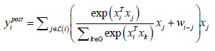
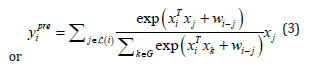
Table 3: Desirable Properties in convolutions and attention that CoAtNet model retains [12].

This configuration retains the property of translation equivariance in convolution, and it retains both the input-adaptive weighting and global receptive fields of self-attention mechanism. Table 3 summarizes the properties that CoAtNet retains from convolutions and attention mechanism (Table 3).

Experimental Setup

The selected CoAtNet variation for this study is CoAtNet-0. We used TensorFlow and Keras platforms to conduct this experiment. The only available pre-trained CoAtNet found in the used platform is CoAtNet-0 as such we adopted it for this experiment. Also, given the fact that it has the smallest number of parameters we anticipate that it would give optimal results given our small dataset. The experiments were conducted in Google Colab Pro+ using the standard GPU NIVIDIA V100. We experimented with a variety of scenarios and compared them. We used both the trained and pre-trained versions of CoAtNet in our experiments. We used cross entropy loss function:

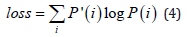
Where P’(i) is ground truth probability and P(i) is predicted probability. The number of epochs is 50. The dataset was expanded and an additional fourth class added, as mentioned in the dataset section. The split of the data is kept as for training and testing where roughly training is 81% and testing is 19%. In addition, 10% of the training dataset was dedicated for validation. The model was trained end-to-end, meaning no layers were frozen during training, in case of fine tuning. The model was initially trained without any augmentations. As we attempt to improve performance, we gradually apply augmentation, and normalization. We also investigated the effect of increasing batch size and implementing a scheduled decaying learning rate.

Normalization

To make convergence faster and training more stable, we utilize input normalization in which the inputs are made to have a mean of 0 and standard deviation of 1.

Augmentation

Augmentation involves the expansion of a dataset by adding transformations or perturbations to a dataset. In our experiments, as mentioned, we began with plain training, that is without any augmentation. Then, we gradually added augmentations to test performance in the sequence mentioned below:

a. Flipping: random horizontal flipping of an image on axis x.

b. Rotation: random rotation with a factor of 0.2.

Increase of Batch Size

The batch size in our experiments was very large. We selected a batch size of 100. According to Samuel, et al., [12] increasing batch size to a large number of increases performance and has a similar effect learning rate decay.

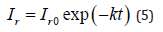
Exponentially Decaying Learning Rate

The learning rate was made exponentially decreasing. The initial rate was set at 0.0001. In the final experiment it was further reduced to 0.000001.

The above techniques will be referred to in this convention: (N) for normalization, (AUG) for augmentation, (LB) for Large Batch Size, and (DLR) for decaying learning rate. The optimizer used throughout all experiments is ADAM optimizer [13].

Results

In the beginning the model was run in plain training where no additional augmentations or learning rate decay were added. Plain training was applied to a pre-trained and a non-pretrained CoAt- Net-0 model. The results showed that pre-trained model outperforms the non-pretrained model, where the first achieved 97% and the latter 88%. Then, we increased the batch size from 1 to 100. The accuracy improved to 97.4%. We decided to add an augmentation (random flipping) to improve performance which resulted in 99.08%. Then, we also add exponential decaying leering rate along with normalization to increase performance. However, the performance dropped slightly, even though we were expecting better results. For this reason, we decreased the initial learning rate to 0.000001. We also made an important observation on the training accuracy. Before applying normalization, we noticed to have some perturbations in the training accuracy. For this reason, we add normalization to smooth out training. The comparison of those two trainings, the one before and the one after normalization is shown in Figure 3. Normalization improved the training profile (Figure 3).

In the last experiment, as mentioned earlier, we decreased the learning rate from 0.00001 to 0.000001. In addition, we added one more augmentation which is random rotation. In total, the augmentations became two. We achieved the higher accuracy in literature which is 99.16%. The table below summarizes our results. The confusion matrix of the best achieved accuracies is shown in Figure 4 in Table 4, we compare our results with previous literature. In Figure 5, we show some samples of output from the model with the highest accuracy (Table 4) (Figure 4).

Figure 3: Comparison between two different types of residual blocks. (a) conventional Residual block, and (b) inverted blocks (used in CoAtNet model and MobileNet-V2).

Figure 4: Confusion matrix for highest performing models. (a) pre-trained + LB + 2AUG + DRL, (b) pre-trained + LB + 1AUG + DLR, and (b) pretrained + LB + 3AUG + DRL.

Figure 5: Samples of classified images. Green indicates correct classification. Red indicated wrong classification.

Table 4: Results of CoaAtnet-0 model and enhancements. The fine-tuned models are pre-trained on Image Net.

Discussion

The results have illustrated the transformative potential of the CoAtNet model in the field of brain tumor classification, charting a path towards a promising future in medical image analysis. The accuracy obtained was 99.16% which is the highest recorded in literature. Though, one may notice that when the model is not pretrained, it achieves quite a low accuracy which is around 88%. Nevertheless, for a big model like CoAtNet, this result is actually considered a breakthrough. As in our experiments, VGG, and Res- Net50 and ResNet101 failed to converge when not pre-trained. In Figure 6, we show a comparison between the trajectories training of a non-pretrained CoAtNet and a non-pretrained ResNet. This behavior proves that CoAtNet has high flexibility even with small datasets which is usually the case in medical imaging. Therefore, it can be a good potential for all future applications, beyond brain tumors, in medical imaging and should replace the choice of ResNet. (Figures 5,6) (Table 5).

Table 5: Comparing results to related literature work.

Figure 6: a comparison between a non-pretrained ResNet and a non-pretrained CoAtNet. (a) ResNet diverges and cannot handle small datasets without pre-training, (b) CoAtNet shows flexibility with small datasets without pre-training.

Conclusion

In In this study, we used the CoAtNet model to classify brain tumors. The model showed potential if pre-trained and certain adjustment such as the addition of augmentations, decaying learning rate, and use of large batch size techniques are implemented. We were able to achieve an accuracy of 99.16% which is higher than state-of-the-art.

Acknowledgement

None.

Conflict of Interest

None.

References

• Cheng J, Yang W, Huang M, Huang W, Jiang J, et al., (2016) Retrieval of brain tumors by adaptive spatial pooling and fisher vector representation. PloS one 11(6): e0157112.
• Francisco Javier Díaz Pernas, Mario Martínez Zarzuela, Míriam Antón Rodríguez, David González Ortega (2021) A Deep Learning Approach for Brain Tumor Classification and Segmentation using a Multi-scale Convolutional Neural Network. Healthcare 9(2): 153.
• Özlem Polat, Cahfer Güngen (2021) Classification of brain tumors from MR images using deep transfer learning. The Journal of Supercomputing 77(7): 7236-7353.
• Afshar P, Plataniotis KN, Mohammadi A (2019) Capsule networks for brain tumor classifications based on MRI images and course tumor boundaries. IEEE Xplore.
• Dosovitskiy Alexey, Luca Beyer, Alxander Kolensikov, Drik Weissenborn, Xiaohua Zhai, et al. (2020) An image is worth 16x16 words: Transformer for IMage recognition at scale: 1-22.
• Sudhakar Tummala, Seifedine Kadry, Syed Ahmad Chan Bukhari, Hafiz Tayyab Rauf (2022) Classification of Brain Tumor from Magnetic Resonance Imaging Using Vision Transformers Ensembling. Curr Oncol 29(10): 7498-7511.
• Rehman A, Naz S, Razzak MI, Akram F, Imran M (2020) A Deep Learning-based Framework for Automatic Brain Tumor Classification usinf Transfer Learning. Ciruits, Systems, and Signal Processing 757-775.
• Zar Nawab Khan Swati, Qinghua Zhao, Muhammad Kabir, Farman Ali, Zakir Ali, et al. (2019) Content-based Brain Tumor Retrieval for MR Images Using Transfer Learning. IEEE.
• Dai Zihang, Hanxiao Liu, Quoc V Le, Mingxing Ta (2021) CoAtNet: Marrying convolution and attention for all data sizes. Advances in Neural Information Processing Systems 34: 3965-3977.
• Mark Sandler, Andrew Howard, Menglong Zhu, Andrey Zhmoginov, Liang Chieh Chen (2018) Mobilenetv2: Inverted residual and linear bottlenecks. Proceedings of the IEEE conference on computer vision and pattern recognition: 4510-4520.
• Kaiming He, Xiangyu Zhang, Shaoqing Ren, Jian Sun (2016) Deep Residual Learning for Image Recognition. Proceedings of the IEEE conference on computer vision and pattern recognition.
• SL Smith, PJ Kindermans, C Ying, QV Le (2017) Don't decay the learning rate, increase the batch size. arXiv preprint.
• Diederik P Kingama, Jimmy Lei Ba (2015) ADAM, A Method for Stochastic Optimization. ICRL.
• Jun Cheng, Wei Huang, Shuangliang Cao, Ru Yang, Wei Yang, et al., (2015) Enhanced Performance of Brain Tumor Classification via Tumor Region Augmentation and Partition. PLoS One 10(10): e0140381.
• Ismael MR, Abdel Qader I (2018) Brain tumor classification via statistical features and back-propagation neural network. IEEE International Conference on Electro/Information Technology.
• Abiwinanda N, Hanif M, Hesaputra ST, Handayani A, Mengko TR (2018) Brain tumor classification in MRI using convolutional neural network. Springer World Congr Med Phys Biomed Eng.
• Pashaei A, Sajedi H, Jazayeri N (2018) Brain tumor classification via convolutional neural network and extreme learning machines. IEEE 8th International Conference on Computer and Knowledge Engineering.
• Phaye SSR, Sikka A, Dhall A, Bathula DR (2018) Dense and diverse capsule networks: making the capsule learn better: 1-11.
• Seetha J, Selvakumar Raja S (2018) Brain tumor classification using convolutional neural networks," Biomed Pharmacol J 11(3): 1457-1461.
• Avşar E, Salçın K (2019) Detection and classification of brain tumours from MRI images using faster R-CNN. Tehnički Glasnik 13(4): 337-342.
• Zhou Y, Li Z, Zhu H, Chen C, Gao M, et al. (2019) Holistic brain tumor screening and classification based on densenet and recurrent neural network glioma multiple sclerosis stroke and traumatic brain injuries. Springer International Publishing, Brainlesion: 208-217.
• Anaraki AK, Ayati M, Kazemi F (2019) Magnetic resonance imaging-based brain tumor grades classification and grading via convolutional neural networks and genetic algorithms. Biocyber Biomed Engineering 39(1): 63-74.
• Gumaei A, Hassan MM, Hassan MR, Alelaiwi A, Fortino G, et al. A hybrid feature extraction method with regularized extreme learning machine for brain tumor classification. IEEE Access 7: 36266-36273.
• Sultan HH, Salem NM, Al Atabany W (2019) Multi-classification of brain tumor images using deep nerual network. IEEE Access 7: 69215-69225.
• Deepak S, Ameer, PM (2019) Brain tumor classification using deep CNN features via transfer learning. Computational Biology: 111.
• Kaplan K, Kaya Y, Kuncan M, Ertunç HM (2020) Brain tumor classification using modified local binary patterns LBP feature extraction methods. Medical Hypothessis 139: 109696.