Computer Simulation of a Forearm Splint Manufactured with FDM 3D Printing Technology

Introduction

The main reason for the development of 3D printed splints is to overcome some issues found with the traditional splinting methods and materials, such as the associated unattractiveness of the material and the impossibility of temporarily removing the splint during checkups or for cleaning the affected area, among others [1,2].

A review work on the use of additive manufacturing technology, mainly in custom orthoses and prostheses for lower limbs, mentioned other applications such as custom wrist splints [3]. Blaya, et al., [4] obtained a splint printed by Fusion Deposition Modelling (FDM) after scanning a patient’s limb and modifying the geometry using available computer software packages. A few barriers which need to be overcome before additive manufacturing can be regularly used in clinical applications have been considered, such as fabrication time [2,5], and the steep learning curve associated with the design process and construction. The design process seems to be a primary limitation for its use in medical practice. A study by Paterson et al. [6] discussed the possibility of a digitalized approach in the fabrication of arm splints using proprietary/customized computer software and 3D printing techniques.

To design a forearm splint, several steps must be considered, such as obtaining the forearm shape from the patient, adapting the splint design to such geometry, verifying that the splint has the necessary strength and finally, the printing process. Moreover, including ventilation holes is an important aspect considered by several authors [1,4,7], mainly to improve transpiration but also to enhance aesthetics. However, one should consider the effect of such holes in the mechanical behavior of the splint. A few studies [5,8,9] have applied Finite Element Analysis to mechanically evaluate the splint design.

A forearm splint can be considered as a first-class lever with three pressure points. The first point, the wrist, is assumed as the axis of the joint, the other two points are the distal and proximal ends of the splint. These ends oppose any force created at the wrist, which can be calculated as 4N [10]. The same assumption can be applied to a full splint covering both sides of the arm. Some authors [11-13], have measured the torque produced by healthy individuals while bending the wrist both during flexion and extension, with values of up to 34 Nm in one individual [12]. These data may be used to compute the force applied by the patient during splint use, considering that an unhealthy patient might not be able to exert more than 48% of the forces mentioned in those studies [14].

Fused Deposition Modelling (FDM) is commonly utilized to manufacture splints and other orthoses [1,3,4]. In this technology, each layer solidifies before the next layer is printed, then the bonding of polymer molecules between layers is not the same as that of molecules deposited during layer printing. This causes a difference in material properties depending on printing direction and whether stresses are applied parallel or perpendicularly to the printed layers [15]. The difference can be of up to 33% in some of the mechanical properties of 3D printed ABS samples [16]. Domingo Espin, et al., [17]. considered 3D printed ABS parts as orthotropic materials and defined the compliance matrix of such materials. The necessary data consisted of: ε_i, the elongation in each of the 3 directions (x, y, z); γ_ij , the shear strain for each plane defined by ij; σ_i , the normal stress; γ_ij , the shear stress. From this data, Young’s modulus (E_i), Poisson’s ratio (v_ij) and shear modulus (G_ij) in each plane were calculated.

A few studies concerning 3D printed splint computer simulation have been found in the literature. The first one [5] described a full flow process regarding the automation of the splint design, including a computer simulation step within the process. ABS was the chosen material, making the following assumptions:

i. the design included a screw closure system which was disregarded in the computer model;

ii. a force of 30N was applied in the distal surface;

iii. the proximal surface was fixed to restrain the model’s movement.

The study concluded that the stress and displacement values for the splint (13.91 MPa y 0.53mm, respectively) were adequate for the design, but no comparison was made with experimental results. The results of [5] also allow the conclusion that both halves of the splint were considered as bonded together, since there does not seem to be any relative movement between them. On the other hand, Lin, et al., [8] performed a computer simulation for a forearm splint and considered the splints’ parts as fully bonded. In their work, the authors only evaluated the impact resistance, without analysing the flexural behaviour. A third computational work [9] included an experimental evaluation of FEA results for a splint design. The splint consisted of a single piece printed out with two different materials, one which was more flexible allowing the splint to open, thus allowing it to be placed or removed from the patient’s forearm. The authors modelled both materials with almost identical values of Young’s modulus (2000 and 2078 MPa, respectively). The splint was fully closed with a series of rubber bands, modelled as idealized springs. Four loading scenarios were used, concluding that for two of them there was a good correlation between experimental results and computer simulations.

Materials and Methods

Our work addressed the main aspects involved in the design and manufacture of a custom 3D printed splint for the forearm, including forearm scanning, cleaning and preparing the geometry, splint design and 3D printing. However, the focus was on a fundamental part of the design process: verifying that the 3D printed splint has an adequate mechanical behaviour when used by the patient, for example, enough rigidity to prevent the forearm from moving during immobilization treatments. The process included mechanical testing of 3D printed material samples, analysis of the constitutive model that describes the material behaviour, modelling of a bending test in a computational software using the geometry of the designed splint and experimental mechanical properties. Finally, the numerical results were compared with an experimental bending test of the 3D printed design.

A useful improvement on previous computational works [5,8] was to consider the different parts of the splint as individual interacting geometries, not necessarily bonded to each other. Furthermore, the three pressure points mentioned in [10] were added to the model and computational results were compared to experimental flexural test results. The contact between the different parts of the splint and between the splint and the flexure apparatus should be taken into consideration. Although analytical equations have been derived for common geometries [18], it is necessary to solve for contact between more complicated geometries such as those found in the human body.

Comsol Multiphysics® (COMSOL Inc., version 5.4, Burlington, MA, USA) was chosen to carry out the computational work, including the contact modelling. Studies by Schupp, et al., [19], Ranjan, et al., [20] and Kumar, et al., [21], among others, exemplify the use of contact mechanics of different complex systems and represent a base for this study.

Scanning and Printing

The geometry of a human forearm was scanned using a Structure Sensor (Mark II) (Occipital Inc., Boulder, CO, USA). The resulting geometrical model was cleaned of unnecessary objects, aligned to the X, Y and Z axes, and transformed into a solid geometry with Autodesk’s Meshmixer (Autodesk Inc., San Rafael, CA, USA). The final modification into the splint design, including the closure system, was performed using SolidWorks (Dassault Systèmes SE, 2019 SP03, Vélizy-Villacoublay, France). Figure 1 shows the end splint design used in the model. It consists of two halves that join using a snap and hook mechanism which can be easily removed to perform medical check-ups, clean-ups, etc (Figure 1).

Figure 1: Geometry of the splint and detail of the snap and hook mechanism.

Figure 2: Necessary printing orientations to obtain mechanical properties for an orthotropic material, (adapted from [17]).

An Ultimaker® FDM printer (Ultimaker B.V., v2, Utrecht, Netherlands) was used to print four different configurations of tensile test samples according to ASTM D638 (Type 4). These samples correspond to configurations 1, 3, 4 and 5, depicted in (Figure 2).

An assumption was made that configurations 5 and 6 should show similar properties, as well as 1 and 2, although for the latter this is not entirely true [17]. The selected material was ABS, with printing parameters reported in APPENDIX 1: Printing parameters.

Tensile and Bending Tests

Five samples for each configuration mentioned in the previous section were printed and a standard tensile test performed according to ASTM D638. The experimental results were fed into a proprietary Matlab function which calculated the different mechanical properties, such as Young’s modulus, elastic limit, elongation, ultimate and fracture strengths, later used then to obtain the values of the shear modulus in all necessary planes. The information was used as an input for the computational model and to compare numerical results with bending test experiments.

The splint parts were printed at a 50% of their real size to obtain a reasonable manufacturing time, then assembled to perform a bending test using a MTS universal testing machine (MTS Systems Corporation, model 370.02, Minneapolis, MN, USA) with a bending fixture according to ASTM D790. It was assumed that the force exerted on the splint depended on the patient and his specific condition. The bending test was executed to failure and maximum applied force and deflection curves were used for comparison with computational results. Before performing the bending test, several pictures were taken to register the exact position of the splint over the bending test fixture. This was made to replicate the relative position between the flexure apparatus and the splint in the computational model, as accurately as possible.

Computer Simulation

Figure 3 represents the layout of the computer model, the splint in the middle and three solid cylinders representing the three contact points in the flexion test fixture. The geometry was scaled to 50% to resemble the actual experimental test. The top cylinder of the geometry was the loading unit of the flexure fixture (Figure 3).

A prescribed displacement node was added to describe the movement of the loading unit along the Y axis during the test, with no displacement on the X or Z axes. This movement was increased from 0 to 6 mm, using steps of 1 mm and will be referred to as “deflection”. The computational model was limited to 6 mm of deflection, due to convergence problems that would arise near the failure limit of the material. Furthermore, the bottom cylinders represented the supports of the fixture and were constrained from movement in all directions but allowing their rotation.

Figure 3: Disposition of geometries for the computer model, the cylinder on top represents the tip of the conical actuator in the flexion test fixture.

The movement of the top cylinder was transmitted to the splint through the contact surface, while the bottom cylinders prevented the movement of the unit. Contact nodes were included between the three cylinders and the splint to be able to calculate the amount of pressure transmitted. For each contact node, the source (or master) boundary was set on the cylinder and the destination (or slave) boundary on the splint surface. An augmented Lagrangian method was used to solve the contact mechanics, with no friction and a preset for stability. The main equations used to solve the contact mechanism are given in Eq. 1, when the gap between contact surfaces is nil or negative and for every other case.

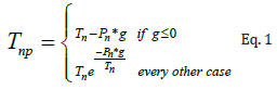
In Eq. 1,T_n is the contact pressure, g is the gap between the contacting surfaces, and P_n is the penalization factor.

Figure 4: Detail of the gap between the two main parts of the splint.

Initially, a contact node was used between all pieces of the splint assembly, but computer memory limitations required some of these nodes to be eliminated. Thus, the whole splint was considered as one piece, with the two main halves separated by slightly altering the geometry to include a gap as shown in Figure 4. As discussed later, this modification is important to obtain a behaviour closer to the experimental flexural test results. The contact force was computed through an integration of the contact pressure calculated by the contact nodes. This procedure was used to evaluate individual forces at the top cylinder and both the bottom cylinders, checking that the sum of all forces is equal to zero (Figure 4).

Two prescribed displacement nodes were added to stabilize the solution and prevent the movement in the X axis, which is perpendicular to the YZ plane of Figure 3. One node was placed on the far top left of the splint and prevented displacement on the X axis only. The second node was added on the far right, avoiding the movement on both the X axis and the Z axis (left to right in Figure 3).

A linear elastic material model was used, and the von Mises stress was calculated for the material of the splint. Due to the test conditions of the study, it was assumed that these models accurately represented the behavior during the bending test. A Poisson’s ratio v value of 0.37 was set for each printing orientations as obtained from literature, where different printing orientations have shown almost the same behavior, with values of v between 0.36 and 0.38 [16]. Finally, for the finite element solution with Comsol Multiphysics®, the cylinders were meshed using the extremely fine mapped mesh which improved the model’s convergence. For the rest of the domains a free tetrahedral mesh was used (Figure 5), giving a total of 96160 finite elements (Figure 5).

Figure 5: Mapped and free tetrahedral meshes used in the computational model of the splint.

Results and Discussion

Tensile and Bending Tests

The tensile test results for the samples of configuration 4 are plotted in Figure 6, with the elastic zone showing little variation. Although the failure limit varies significantly, the model describes the material behavior only in the elastic zone (Figure 6).

Figure 7 plots the tensile test data for the samples of configuration 6 representing the behavior of the material under forces perpendicular to the XY plane, along the Z axis. These specimens, which were more difficult to print due to their orientation, exhibit a higher variability in both their elastic and failure behavior, but still within reasonable limits (Figure 7).

Figure 6: Tensile test measurements for ±45° printed samples.

Figure 7: Tensile test measurements for samples printed along the Z axis.

Table 1: Mechanical properties used for the computer simulation of the splint. Including Ei (Young’s modulus), Gij (shear modulus) and the failure limit in the Z direction.

Table 1 gives the mechanical properties measured by testing the experimental samples and later used in the computational model of the splint. According to [17], the required values of (Young’s modulus) and (shear modulus) were calculated from tensile tests performed with specimens as follows: and from specimens printed at alternated 45° angle traces, equal to configuration 4 of Figure 2; calculated from specimens printed at alternated 90° angle traces, equal to configuration 1 of Figure 2; evaluated from tensile tests performed with specimens printed along the Z axis, according to configuration 3 of Figure 2; and computed from specimens printed at a 45° angle from the Z axis, likewise to configuration 6 of Figure 2 (Table 1).

The experimental results show that all magnitudes are slightly higher than what was found in literature but within reasonable limits. For example, in [16] values of around 1960 MPa were given for E_x and E_y, and of 770 MPa and 670 MPa for G_xy and G_yz , respectively. The largest difference is encountered for the value of i>E_z, which in [16] was around 2040 MPa compared to 1311.67 MPa of this work. Both studies have used a FDM printer of the same model, but the difference in printing parameters might affect the calculated properties [22], particularly the values of the layer height (0.1 mm in [16] and 0.2 mm in this work). Also, extrusion and printer bed temperatures might influence as well, but they were not reported in the previous study (Figure 8).

Figure 7: Flexural test results.

Figure 9: Detail of the failure zone during the flexural test.

The results of the flexural test are plotted in Figure 8 and a detail of the failure is shown in Figure 9. We observe how the top half of the splint deforms and overlaps the bottom half during the test. This relative movement is critical and initially explains why the splint halves cannot be considered bonded to each other in the computational model. During the flexure test, the splint failed in the zone just below the loading unit of the fixture (Figure 9). To analyze this failure, the Z failure limit was calculated to compare it with the Z component of the von Mises stress given by the computer model (Figure 9).

The maximum load applied before failure (around 140N) clearly exceeds the loads of [4] (4 N), [8] (30 N) and [9] (11.90 N). Although these loads were applied in slightly different scenarios, the measured maximum load suggests that the proposed design is strong enough for its application. Therefore, ventilation holes might be added for a future improvement of the design while still maintaining adequate rigidity for its intended use. In that case, topological optimization techniques might be included for future evaluations of materials and design [23].

The closure system behaved adequately during the test and transmitted the forces from one half of the splint to the other. One of the closure pieces moved slightly during the test (bottom left corner of Figure 9) due to a printing defect which was not spotted during the assembly process of the splint. A modification of the design might improve the ease of printing of these pieces, eliminating overhangs and replacing them with angled or sloping walls as shown in (Figure 10).

Figure 10: Detail of the modification for the closure mechanism, eliminating overhangs at the left.

Computational Results

For a deflection of 6 mm, Figure 11 shows the von Mises stress distribution with values lower than 50 MPa along most of the geometry. However, when dealing with non-isotropic materials, the components of stress in the different directions should also be considered (Figure 11).

Figure 11: Von Mises stress for a 6 mm deflection, as computed by the computational model.

Figure 12: Detail of the displacement for a deflection of 6 mm, showing how the top half of the splint bends and overlaps the lower half in the computational model.

Figure 12 gives a detail of the zone where the top half overlaps the bottom half of the splint, confirmed by the flexural test of Figure 9. As mentioned earlier, this result confirms that it is fundamental to model the geometry as separated interacting parts. Results of previous studies [5,8], do not seem to exhibit this behaviour, which would indicate that the geometry was instead modeled as a single part (Figure 12).

Figure 13 and Figure 14 give the splint displacements for a deflection of 6 mm. These results clearly show how the top half will overlap and deflect more than the bottom half when considered as separated pieces. The top cylinder is shown in red since it matches the total (maximum) deflection exactly (Figures 13,14).

Figure 13: Displacement values (mm) in the splint for a deflection of 6 mm.

Figure 14: Displacement values (mm) in the splint for a deflection of 6 mm, bottom view.

The detail of Figure 9 indicates that the failure during the flexion test occurred in the XY plane and along the Z axis. Then, the Z component of the von Mises stress is compared to the failure limit in the Z direction and the result is shown in Figure 15, showing in red the zones where the calculated stress is above the limit. Variables such as printing defects, among others, will determine the exact location of the failure in the experimental test. The results show a similarity betweenthe red zone at the center of the top piece of the splint (Figure 15) and the failure zone observed in Figure 9 during the flexural test. Similar comparisons for the X and Y directions highlight that the failure limit is exceeded only in the Z direction and very slightly in the X direction, in the zone right under the top cylinder, quite similar to Figure 9. This is expected, since the splint flexes mostly along the Z axis, which also has the lowest mechanical properties, increasing the tension there. It could be compensated by increasing the thickness of the splint, but as mentioned earlier, the failure load was more than enough for the intended application (Figures 15,16).

Figure 15: Comparison of the Z failure limit (7.91 MPa) with the von Mises stress Z component, for a deflection of 6 mm. A value of 1 (shown in red) indicates the von Mises stress is higher than the failure limit in that zone.

Figure 16: Total contact force for both the upper and lower cylinders for each deflection step.

Figure 16 plots the total calculated force load, revealing three main characteristics. First, the force on the upper cylinder and that of both the lower cylinders is the same, with a minimal difference that might be attributed to computational approximations, indicating that the sum of forces is in fact zero. The general trend of the curve is close to that observed in the flexural test, although the force is higher for each deflection value. This could be explained by the fact that the contacts between the splint and the closure mechanism parts were fixed (bonded) for the computational model, which can cause it to be slightly more rigid and, hence, requiring more force to bend. In fact, the deflection at which the Z axis stress limit is initially reached is 3 mm (Figure 17).

As seen in Figure 16, the total force calculated at a deflection of 3 mm was around 140 N, close to the resulting force at failure of the flexural test. Again, this would indicate that for the same force less deflection is observed, with the modelled splint slightly more rigid than expected. A further study might include a more appropriate non-linear material model and modified von Mises criteria to improve the results according to the failure modes for each of the printing directions, similar to the elastoplastic constitutive model proposed by Wang, et al., [24] for SLA printed materials.

Figure 17: Comparison of the Z failure limit with the von Mises stress z component, for a deflection of 3 mm. A value of 1 indicates the von Mises stress is higher than the failure limit in that zone.

Conclusions

In this work a flexion test has been performed for a 3D printed splint design and tension experiments have been carried out to obtain mechanical properties of ABS 3D printed specimens. The maximum load during the flexural test of the splint has shown that the device could withstand forces above those needed for its intended application. Only a slight modification to the snap and hook closure system was suggested to improve the 3D printing process, although it has behaved adequately during the test.

The properties calculated from the tension tests have been used for a finite element model of the splint to simulate its performance during the flexion test. The complexity of the interaction between all the different parts of the splint required the computational model to be validated with experimental results. Comparison between computer simulations and flexural experiments have indicated that considering this mechanical interaction is necessary to obtain a satisfactory computational model.

A few limitations have been found due to the complexity of the geometry and the STL format used to import it into the CAD/CAM program, such as difficulties to improve the meshing in the main body and closure system contact zones, needed to enhance the convergence of the contact numerical computation. However, the overall results are quite satisfactory and might be helpful in the design of future splints, maybe including topology optimization for ventilation holes, overall geometry and thickness of this device.

Acknowledgement

The authors would like to acknowledge the support from the Research and Extension Vice-Rectory of the Costa Rica Institute of Technology (ITCR) through the project n. 1490020, and the ITCR Master Program in Medical Devices Engineering.

Conflict of Interest

The authors declare that they have no known competing financial interests or personal relationships that could have appeared to influence the work reported in this paper.

Standard Test Methods

1. ASTM D638-14 Standard Test Method for Tensile Properties

2. ASTM D790-10 Standard Test Methods for Flexural Properties of Unreinforced and Reinforced Plastics and Electrical Insulating Materials

Appendix 1: Printing Parameters

The printing parameters for the tensile samples were set as follows:

i. Nozzle size: 0.4mm.

ii. Nozzle temperature: 260°C.

iii. Bed temperature: 110°C.

iv. Print speed: 15 mm/s for first and last layers, 25 mm/s for the rest.

v. Raft support.

vi. Air gap: 0.3mm.

vii. Layer thickness: 0.1mm.

viii. A wall count of 2, 0.4mm thickness for each.

ix. 100% infill.

x. Infill directions alternated at -45/+45 degrees relative to the X axis.

xi. All other parameters set by default in Ultimaker Cura software.

For the splint and closure system, the same parameters were used except for the air gap which had to be lowered to 0.1mm and the fan speed which was lowered to 30% for the first 5 mm of printing, this due to adhesion problems which arose during printing.

Appendix 2: MATLAB Function

% program start

tic

clear all

close all %closes any other plots which might be open

archivo = 'Z45-5.dat';

fileID = fopen(archivo,'r');

lo=72;

Area=24.042222;

porcentajeLimElastico=0.02; %percentage for elastic limit calculation, normally 0.2% but in this case 0.02% gave the best results

angulocaida=89.995; %angle to determine fracture point, a lower value will bring the fracture point closer to the ultimate strength

A = fscanf(fileID,'%c');

fclose(fileID);

n=length(A);

y=1;

t='';

count=0;

x=1;

for i=1:n

%Ai=A(i)

%p=i

if count>7 && count<2056 %counter to avoid file headings

%Ai=A(i)

t=strcat(t,A(i)); %

if A(i)==' ' %If A(i) a “space”

%t=t

if length(t)>0 %sometimes the file has 2 “space” one after the other

if y== 1

B(x,y)=str2num(t)/lo;

else

B(x,y)=str2num(t)/Area;

end

y=y+1;

t='';

end

end

if A(i)==char(13) %If A(i) is an “Enter” or line break

y=1;

x=x+1;

t='';

end

end

if A(i)==char(13) % If A(i) is an “Enter” or line break

Aimenos1=A(i-1);

count=count+1;

end

if count==2056% counter to avoid file headings

%resets to zero when it gets to 2056 and

%avoids next heading

count=0;

end

end

%B=[B(:,1)/lo B(:,2)/Area] %transforms B to strain and stress

Xlineal=[1 B(1,1);1 B(2,1)];

Btemp=[B(1,2);B(2,2)];

rMax=0;

for i=3:length(B(:,1))

Xlineal=[Xlineal;1 B(i,1)];

Btemp=[Btemp;B(i,2)];

regresion=Xlineal\Btemp;

aproxlineal=Xlineal*regresion;

r2=1-sum((Btemp-aproxlineal).^2)/sum((Btemp-mean(Btemp)).^2);

if r2>rMax

moduloyoung=regresion;

rMax=r2;

end

end

[LimMax,I] = max(B(:,2));

lineaYoung=(B(:,1)-porcentajeLimElastico/100)*moduloyoung(2);

i=1;

while lineaYoung(i)<B(i,2)

%compares the current stress value with the same position in Youngs limit line

%when Youngs limit line value is bigger than the current stress

%the previuos stress and strain values are stored as values for the elastic limit

enlonglimelastic=B(i,1);

limelastic=B(i,2);

i=i+1;

end

i=I; %point i starts at the ultimate limit, to calculate the fracture point from there on dif=0;

while (i<length(B(:,1))-15) && dif<tand(angulocaida)

% calculates difference in the stress value for point i and another point i+15, and stops as soon as the angle between point i and point i+1 is less than stablished by variable “angulocaida”

dx=B(i+15,1)-B(i,1);

dy=B(i+15,2)-B(i,2);

dif=abs(dy/dx);

limultimo=B(i,2);

enlonglimultimo=B(i,1);

i=i+1;

end

clf

hLine = plot(nan); %# starts a plot without any data and calls it "hLine"

axis([0 max(B(:,1)) 0 round(LimMax,1)+1]) %calculates limits for x and y axis

set(hLine,'XData',B(:,1)); %specifies x values for the plot (XData)

set(hLine,'YData',B(:,2)); %specifies y values for the plot (YData)

xlabel('Deformación')

ylabel('Esfuerzo (MPa)')

hold on

plot(B(:,1),lineaYoung)

hold on

plot(enlonglimultimo,limultimo,'xr') %puts the red 'x' on the fracture point

drawnow

Resultados = {'Probeta' archivo;

'Módulo de Young' num2str(round(moduloyoung(2),2));

'Límite elástico' num2str(round(limelastic,2));

'Enlongación en el límite elástico' num2str(round(enlonglimelastic,4));

'Límite máximo' num2str(round(LimMax,2));

'Enlongación en el límite máximo' num2str(round(B(I,1),4));

'Límite último' num2str(round(limultimo,2));

'Enlongación en el límite último' num2str(round(enlonglimultimo,4))};

T=table(Resultados)

tiempo=toc;

%program end (Figure 18)

Figure 18: Stress-Strain graph for sample Z-4 obtained using the Matlab function. The gradient of the red line represents Young’s modulus, and the red cross shows the calculated fracture point.

References

• S Kelly, A Paterson, R Bibb (2015) A Review of Wrist Splint Designs for Additive Manufacture, in: Rapid Design, Prototyping and Manufacture Conference, Loughborough, Great Britain.
• A Paterson, R Bibb, RI Campbell (2012) Evaluation of a digitized splinting approach with multiple-material functionality using Additive Manufacturing technologies, 23^rd Annual International Solid Freeform Fabrication Symposium - An Additive Manufacturing Conference, SFF: 656-672.
• RK Chen, Y Jin, J Wensman, A Shih (2016) Additive manufacturing of custom orthoses and prostheses—A review. Additive Manufacturing 12: 77-89.
• F Blaya, PS Pedro, JL Silva, R D’Amato, ES Heras, et al. Design of an Orthopedic Product by Using Additive Manufacturing Technology: The Arm Splint J Med Syst 42(3): 54.
• J Li, H Tanaka (2018) Rapid customization system for 3D-printed splint using programmable modeling technique - a practical approach. 3D Print Med 4(1): 5.
• AM Paterson, E Donnison, RJ Bibb, R Ian Campbell (2014) Computer-aided design to support fabrication of wrist splints using 3D printing: A feasibility study. Hand Therapy 19(4).
• YJ Chen, H Lin, X Zhang, W Huang, L Shi, et al. (2017) Application of 3D-printed and patient-specific cast for the treatment of distal radius fractures: initial experience. 3D Print Med 3(1): 11.
• H Lin, L Shi, D Wang (2016) A rapid and intelligent designing technique for patient-specific and 3D-printed orthopedic cast. 3D Print Med 2(1): 4.
• A Cazon, S Kelly, AM Paterson, RJ Bibb, RI Campbell (2017) Analysis and comparison of wrist splint designs using the finite element method: Multi-material three-dimensional printing compared to typical existing practice with thermoplastics. Proc Inst Mech Eng H 231(9): 881-897.
• RM Duncan (1989) Basic Principles of Splinting the Hand. Phys Ther 69(12): 1104-1116.
• RV Gonzalez, TS Buchanan, SL Delp (1997) How muscle architecture and moment arms affect wrist flexion-extension moments. J Biomech 30(7): 705-712.
• JM Vanswearingen (1983) Measuring Wrist Muscle Strength. J Orthop Sports Phys Ther 4(4): 217-228.
• Y Yoshii, H Yuine, O Kazuki, W Tung, T Ishii (2015) Measurement of wrist flexion and extension torques in different forearm positions. Biomed Eng Online 14: 115.
• AA Amis, S Hughes, JH Miller, V Wright, D Dowson (1979) Elbow Joint Force in Patients with Rheumatoid Arthritis. Rheumatol Rehabil 18(4): 230-234.
• F Calignano, D Manfredi, EP Ambrosio, S Biamino, M Lombardi, et al. (2017) Overview on Additive Manufacturing Technologies. Proceedings of the IEEE 105.
• J Cantrell, S Rohde, D Damiani, R Gurnani, L DiSandro, et al. (2017) Experimental Characterization of the Mechanical Properties of 3D Printed ABS and Polycarbonate Parts. in.
• M Domingo Espin, JM Puigoriol Forcada, AA Garcia Granada, J Llumà, S. Borros, et al. (2015) Mechanical property characterization and simulation of fused deposition modeling Polycarbonate parts. Materials & Design 83: 670-677.
• VL Popov, M Heß, E Willert (2019) Handbook of Contact Mechanics. Springer Berlin Heidelberg.
• G Schupp, C Weidemann, L Mauer (2004) Modelling the Contact Between Wheel and Rail Within Multibody System Simulation. Vehicle System Dynamics 41.
• R Ranjan (2019) How to Model a Cam Follower Mechanism.
• C Kumar (2019) How to Model the Compression of a Hyperelastic Foam.
• J Kotlinski (2014) Mechanical properties of commercial rapid prototyping materials. Rapid Prototyping Journal 20.
• A Zolfagharian, TM Gregory, M Bodaghi, S Gharaie, P Fay (2020) Patient-specific 3D-Printed Splint for Mallet Finger Injury. Int J Bioprint 6(2): 259.
• S Wang, Y Ma, Z Deng, K Zhang, S Dai (2020) Implementation of an elastoplastic constitutive model for 3D-printed materials fabricated by stereolithography. Additive Manufacturing 33: 101104.