Research Article 
![]() Creative Commons, CC-BY
Creative Commons, CC-BY
Comparison of Some Variable Selection Techniques in Regression Analysis
*Corresponding author: Obubu Maxwell, Department of Statistics, Nnamdi Azikiwe University, Awka, Nigeria.
Received: November 13, 2019; Published: November 26, 2019
DOI: 10.34297/AJBSR.2019.06.001044
Abstract
In this research, we analyze critically the performance of four variable selection techniques in the building of a model that best estimate a dependent variable. The variable selection techniques are the direct search on t method, the forward selectio
n method, the backward elimination method, and the stepwise regression method. To compare, an economic data of 32 years was collected each on Real Gross Domestic Product, which was the dependent variable used as a measure for economic growth and development, and seven factors which are; Growth Market Capitalization, All-shares index, the Market turn-over, the openness of the Nigerian trade economy, the value of transaction, the total listing of the Nigeria stock exchange, and total new issue. Regressing the Real gross domestic product on the seven factors using the four variable selection techniques, the residual mean square, adjusted R2, and variance inflation factor obtained from the use of each of these techniques which are the criteria for evaluation of best model were compared by ranking them based on the method best satisfying the criteria for evaluation. The result shows that with a mean rank of 1.67 taken across the criteria, the backward elimination method performs best in variable selection based on the sample collected and it supported with the use of the all possible combination method as a control.
Keywords: Variable Selection Technic; Regression Analysis; Backward Elimination Method; Stepwise Regression; Growth Market Capitalization; All-Shares Index; Market Turn-Over; Real Gross Domestic Product
Introduction
Regression is a very powerful tool that explains a variable using other independent variables. But in real life a certain variable is influenced by enumerable number of factors. Some are measurable and others immeasurable; for example, income, agriculture, the economy, student’s performance etc. Some of these factors are significant, while others are less significant, since it is not possible to account for all the variations in a certain factor (Independent variable). So, it is necessary to select variables whose influence on the dependent variable is relatively more significant. In a situation where there is a pool of candidate regressors that should include all the influential factors, but the actual subset of regressors that should be used in the model needs to be determined [1]. Finding an appropriate subset of regressors for the model is called variable selection problem and it requires the use of some variable selection techniques, techniques such as; Direct Search on t Statist ics, the Backward Elimination method, the Forward selection method, Stepwise Regression method, and the All Possible Combination method.
Building a regression model that includes only a subset of the available regressors involves two conflicting objectives; To build a model that would include as many regressors as possible so that the information content in these factors can influence the predicted value of the dependent variable, and to build a model that would include as few regressors as possible because the variance of prediction increases with variance in the number of regressors. Though the building of the model having too many regressors may not be preferred because of it entails greater cost of data collection and model maintenance. The process of finding a model that is a compromise between these two objectives is called selecting the “Best” regression equation. In a situation where all method gives different equation as the appropriate subset model for estimation, then the mean rank method of choosing the best will be applied; that is, the method will be ranked based on the criteria used. This will be applied to choose the best model for All-possible regression method. Here, an estimation of the Nigeria economic growth is to be obtained using the Nigerian Gross Domestic Product as a measure for growth and development, and seven (7) factors that influences its growth will be considered here; factors like the Nigerian growth market capitalization, the Nigerian All-Share Index, Total Listing on the Nigerian Stock Exchange, Total New Issues, Openness of Nigeria Trade Economy, Value of Transactions, Total Market Turnover.
One of the major problems in the use of the various variable selection techniques is that sometimes the techniques do not give the same subset models as the appropriate model. In such cases, where different methods have different subset regressors and each of the regressors in these models have their various contributions to the estimation of the dependent variable. Therefore, there is need to know which of this model obtained from the various variable selection technique is best for estimation. The objectives of the study includes; To obtain the best equation for the estimation of the Nigerian Gross Domestic Product using all variable selection technique, to find out if all the variable selection techniques used, would give the same subset regressor model as the best model, to compare the best equation given by these techniques, using their residual mean square and adjusted as a criteria, and to use the analysis obtained in this research to make recommendations on the various variable selection techniques. The use of All-possible method is not cost effective and it takes time to conduct. It is impractical for problems involving more than a few regressors and it also require the availability of high-speed computers that can develop efficient algorithm for it. This analysis is conducted in order to enlighten researchers and students who conduct regression analysis, where they have to obtain the best subset regressor for estimating a given dependent variable, of the use of other variable selection methods, and probably at the end of this work would be able to show them which of these techniques is better and more reliable. This analysis is also aimed at enlightening students or young researchers of the use of mean ranks, where the need for comparison of best performing method is required.
Literature Review
There have been a growing concerns and controversies on the best variable selection techniques in regression analysis [2, 3, 4, 5, 6, 7, 8] .There existed mixed results among them. Some were of the view that the use of forward selection method is better than the use of backward elimination method based of their findings, some were of the view that the method is outdated thereby bringing about better method of model building and variable selection. While some were of the view that their performance is the same. Fan and Li [4] In a study stated that a good understanding of stepwise method require an analysis of the stochastic errors in the various stages of the selection problem, which is not a trivial task. Richard[3] In a study to investigate four medical variable selection techniques: forward selection method, backward elimination method, stepwise regression method and the All subset combination method. He conducted an analysis on obtaining the best subset model among eight independent variables; chest, stay, Nratio, Culture, Facil, Nurse, Beds, and Census and his findings was that all the techniques gave the same subset models as best model except forward selection.
Guyon and Elisseff (2003) Argued that forward selection is computationally more efficient than backward elimination to generate nested subset of variables and cases when we need to get down to a single variable that work best on its own backward elimination would gotten rid of. Kira and Rendell [8] Argued that weaker subset are found by forward selection, because the importanct of variable is not assessed. This was illustrated with the use of an example where one variable separates the two classes better by itself than either of the two other ones taken alone and will therefore be selected first by forward selection. At the next step, when it is complemented by either of the two other variables the resulting class separation in two dimensions will not be as good as the one obtained jointly by the two variables that were discarded at the first step. And concluded that backward elimination method may outsmart forward selection by eliminating at first stage, the variable that by itself provides the best separation to retain the two variables that together perform best[9, 10, 11]. Bruce (2009) In a study tore-examine the scope of the literature addressing the weakness of variable selection methods and to re-enliven a possible solution of defining a better performing regresson model. And after his study concluded that, finding the best possible subset of variables to put in a model has been a frustrating exercise.
He said many variable selection methods exist and many statisticians know them, but few know they produce poorly performing models. He also said that resulting variable selection methods are a miscarriage of statistics because they are developed by debasing sound statistical theory to a misguided pseudo-theoretical foundation. And he quoted “I have reviewed the five widely used variable selection methods, itemized some of their weaknesses, and described why they are used. I have then sought to present a better solution to variable selection in regression: The Natural Seven-step Cycle of Statistical Modelling and Analysis. I feel that newcomers to Tukey’s EDA need the seven-step Cycle introduced within the narrative of Tukey’s analytic philosophy. Accordingly, I have embedded the solution within the context of EDA philosophy”. Selena [5] In a study of reviewing methods for selecting empirically relevant predictors from a set of N potentially relevant ones for the purpose of forecasting a scalar time series, using simulations to compare selected methods from the perspective of relative risk in one period ahead forecasts[12, 13, 14].
Research Methodology
Sources of data
Secondary sources of data were employed for this study. These include Nigerian Stock Exchange Fact Books, the Nigerian Stock Exchange Annual Reports and accounts (for various years), Central Bank of Nigeria Statistical Bulletins, Federal Office of Statistics Statistical Bulletin. The variables used covers 1981 to 2013 annually on Nigerian Stock Market, which was based on their authenticity and reliability. Using the gross domestic product as the dependent variable and the independent variable are; Growth of Market Capitalization, Total new issues, Total Value of Transactions, Total Listed Equities and Government Stock, Total Market Turnover, All-share index and openness of the Nigerian Economy. Available economic theories were also examined for theoretical support.
Limitations of the data
When talking of the impact of the Nigerian stock market on her economic development, there are many factors and determinants to consider. As such the study was limited and data was collected on only seven of the factors due to consistency and availability of data on yearly basis.
Data presentation: (Table 1)

Table 1: Annual Report of the Nigerian Stock Exchange.
Model specification
In line with the above specification, the research model is specified thus:
a
GDP=f (GMC, ASI, TLNSE, TNI, OOTE, VALTRANS, TNOV)
Where
GDP= Gross Domestic Product
GMC=Growth of Market Capitalization
ASI=All-Share Index
TLNSE= Total Listing on the Nigerian stock Exchange
TNI= Total New Issues
OOTE=Openness of Nigerian Trade Economy
VALTRANS= Value of Transactions
TMT=Total Market Turnover
Methodology
In this analysis, there are more than one independent variable and one dependent variable, and the interest is to determine the subset model that best estimates the dependent variable, Real GDP; such analysis is called the variable selection technique in Regression analysis. Under this analysis, we have various subtopics which we will be exploiting given to the fact that they are required in this analysis.
Correlation Theory: Correlation is an indication of the strength of linear relationship between two random variables. The degree of relationship connecting more than one variable is referred to as multiple correlations. Correlation may be linear when all points (X, Y) on the scatter diagram seem to cluster near a straight line. If all points in the scattered diagram seem to lie near a line, the relationship is linear. Two variables may have a positive correlation, negative correlation or maybe uncorrelated. Two variables are said to be positively correlated if they tend to change together in the same direction, that is, if they decrease or increase together. Two variables are said to be negatively correlated if they tend to change in opposite direction, that is, when one increases, the other decreases and vice versa. Two variables are said to be uncorrelated or to have no correlation if they are not necessarily independent on each other.
The Pearson Product Moment Correlation Coefficient between X and Y can be expressed as;
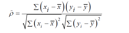
Where ρ is the popul ation correlation, xi and yi are the ith observation of the two variables of interest. While x and y are the mean of the ith observation of the two variables of interest.
Regression Theory: Regression is a statistical tool for evaluating the relationship between one or more dependent variables x1,x2,x3,…xn and a single continuous dependent variable Y. it is most often used when the independent variables are not controllable, that is, when collected in a sample survey or other observational studies. There are so many types of regression model, but just one of the regression models will be used for this study and that is the linear regression model.
Linear Regression Model: A regression model is linear if and only if a variable is a function of another variable whose power equals ones. There are two types of linear regression, and they are; the simple linear regression and the multiple linear regression. For the purpose of the analysis, just the multiple regression will be considered.
Multiple Linear Regressions: Multiple linear regression is a statistical analysis that fits a model to predict a dependent variable from some independent variables. Multiple regressions involve more than one independent variable. The relationship between the dependent and independent variable is expressed as follows:
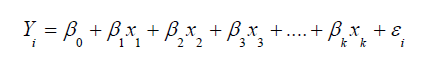
Where
yi is the ith response or dependent variable
xi is the ith independent variable
 is the error term of the ith observation, which is normally,
independently distributed with mean zero and variance
is the error term of the ith observation, which is normally,
independently distributed with mean zero and variance 
β0 β1 β2 β3 βk are the observation parameter.
Estimation of Parameters of the Model: Unbiased estimates of the parameters
β0 β1 β2 β3 βk can be obtained by several methods.
The most widely used is the method of least squares. This
means that the sum of the square’s deviation of the observed
values of Y from their expected value is minimized. In other
words, by the method of least squares, sample estimates of 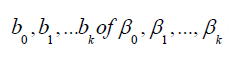 respectively are selected in such a way
that 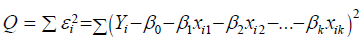 is minimized. As
in simple regression, we obtain estimates, b0, b1….bk of the regression
coefficients by solving the following set of normal equations
is minimized. As
in simple regression, we obtain estimates, b0, b1….bk of the regression
coefficients by solving the following set of normal equations
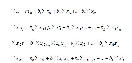
Although these normal equations are obtained mathematically by finding estimates b0, b1, b2, …bk that would minimize equation Q, a simple procedure to remember in obtaining them is as follows: The usual regression equation is written down with b0,b1,…bk as coefficients. The first normal equation is then obtained by summing each term of this regression equation. The second normal equation is obtained by multiplying every term in the regression equation by Xi1 and summing the result. The third normal equation is obobtained by multiplying every term in the regression equation by Xi2 and summing the result; and so on. It will be too cumbersome to obtain separate expressions for the estimates b0, b1, …bk. Instead these coefficients are obtained by calculating the required sums from the data for the various combinations of X1, X2, …and X k and substituting this sum into the normal equations, which are solved simultaneously.
Assumptions of The Regression Analysis: The following are the assumptions of the regression analysis above:
a) X values are fixed in repeated sampling.
b) Zero mean value of disturbanceUI. Given the value of X, the mean, or expected value of the random disturbance term UIis zero. Symbolically, we have E (μi /Xi ) = 0 .
c) Homoscedasticity or equal variance of . Given the value of X, the variance of is the same for all observations. That is, the conditional variances of are identical.
d) No autocorrelation between the disturbances. Given any two X values, and (i≠j) is zero.
e) Zero covariance between i μ and i X , or E (μiXi ) = 0
f) The number of observations n must be greater than the number of parameters to be estimated.
g) Variability in X values. The X values in each sample must not all be the same.
h) There is no perfect multicollinearity. That is, there are no perfect linear relationships among the explanatory variable.
i) The error term is normally distributed, that is,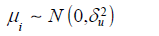
Hypothesis testing: In hypothesis testing there are two types: Null hypothesis and Alternative hypothesis. Null hypothesis is the hypothesis being tested. It is often formulated with the purpose of being rejected. It is stated
as:H0 : β = 0 which shows that the coefficients are the same. Alternative
hypothesis is the hypothesis that contradict the null hypothesis.It is stated as 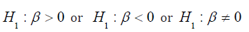 Shows that the coefficients are not the same.
Homoscedasticity: Observations are said to be homoscedastic if they have equal or constant variance. Since one of the assumptions of regression is that the residuals have constant variance, we would be using a scatter plot of the standardized predictors to reach a conclusion on homoscedasticity.
Autocorrelation: The term autocorrelation may be defined as correlation between members of series of observations ordered in time, that is, time series data or space/ cross sectional data. The most celebrated test for detecting serial correlation is that developed by statisticians Durbin and Watson d statistic. A great advantage of the d statistic is that it is based on the estimated residuals, which are routinely computed in regression analysis. However, Durbin and Watson were successful in deriving a lower bound dl and a upper bound du such that if the computed d lies outside these critical values, a decision can be made regarding the presence of positive or negative serial correlation. Moreover, this limit depends only on the number of observations n and the number of explanatory variables. The limits, for n going from 6 to 200 and up to 20 explanatory variables have been tabulated by Dublin and Watson and the limits of 0 and 4.
a) Test of hypothesis: H0 : There is no autocorrelation; 1 H : There is autocorrelation.
b) Decision: Reject the null hypothesis if the Durbin- Watson d statistics value falls outside the limit of d, that is, within the range of 0 and 4.
Level of Significance: The level of significance is the difference between the percentage required and 100 percent. For instance, if 95% certainly is required, then the level of significance will be denoted as α = 0.05. This is the probability of committing a type one error, while a type one error is simply rejecting a true null hypothesis.
Test for Model Adequacy: (Table 2) Test of Hypothesis:H0 :The model is not adequate; H1 : The model is adequate. Using a 5% level of significance.

Table 2: Test for Model Adequacy.
a) Test Statistic: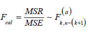
b) Decision Rule:Reject accept if otherwise
Test for Parameter Significance: This is simply a test of the significance of the individual parameters in the model.
a) Test of hypothesis: H0 : β = 0 (The coefficient is not
statistically significant);H1 : β ≠ 0 (The coefficient is statistically significant). Using a 5% level of significance
b) Decision Rule: Reject  accept if otherwise.
Critical Region: Critical region indicates the value of the test statistic that will imply rejection of the null hypothesis. It is also called the rejection region. Opposite of the critical region is the acceptance region, which indicates the value of the test statistics that will imply acceptance of the null hypothesis.
Multicollinearity: Multicollinearity is used to denote the presence
of linear or near linear dependence among the explanatory variables. Multiple regression
model with correlated explanatory variables indicate
how well the entire bundle of predictors predicts the outcome
of the variable, but it may not give valid results about any individual
predictor or about which predictors are redundant
with others. We have a perfect multicollinearity if the correlation
between two independent variables are equal to +1 or -1,
such that we have exact linear relationship if the following condition is satisfied:  . But if
the X variables are intercorrelated to the Y variables, we have:
. But if
the X variables are intercorrelated to the Y variables, we have:  .Where α is the constant, is the
random term, and represents the independent variables with i=
1,2,3, …, k.
.Where α is the constant, is the
random term, and represents the independent variables with i=
1,2,3, …, k.
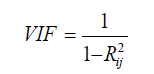
Multicollinearity Diagnostics: Several techniques have been proposed for detecting multicollinearity, but here three techniques will be considered. The desirable characteristics of a diagnostic measure are that it directly reflects the degree of the multicollinearity problem and provide information helpful in determining which regressors are involved. We have; the examination of the correlation matrix, the variance inflation factors, the eigensystem analysis of X’X. Here the variance inflation factor was used to account for the effect of multicollinearity on the various subset regression model.
Variable Selection Techniques: It is desirable to consider regression models that employ a subset of the candidate regressor variables. To find the subset of variables to use in the final equation, it is natural to consider fitting models with various combinations of the candidate regressors. There are several computational techniques for generating subset regression models, but our concentration would be based on four of these techniques and they are; All possible Regressions, Direct Search on t, Forward Selection method, backward elimination method, and the stepwise regression.
All Possible Regressions: This procedure requires that the analyst fit all regression equations involving one candidate regressor, two candidate regressors and so on. These equations are evaluated according to some suitable criterion and the best regression model selected. If we assumed that the intercept term β0 is included in all equations, if there are k candidate regressors, there are 2k total equations to be estimated. For the appropriate model, we consider the adjusted R2 which result is insensitive to the number of variables in the model making it appropriate for decision making in this method where we have to choose the best model combination from the various model combinations, but also the size of the model, that is, the number of variables in the model should also be taken into consideration because the more the variables the more the information obtained from these factors, which actually has a strong influence on the predicted value of independent variable. Though one needs to be careful as to the statement made with respect to the size, because the more the variable the higher the variance of the prediction.
Direct search on t: The test statistics for testing for the full model with p=K+1 regressors is:
 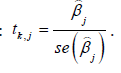 Regressors that contribute significantly
to the full model will have a large
Regressors that contribute significantly
to the full model will have a large  and will tend to be
included in the best p-regressor subset, where best implies minimum
residual sum of squares or Cp. Consequently ranking the reregressors
according to decreasing order of magnitude of the /t k j
/ j=1,2, …, k, and then introducing the regressors into the model
one at a time in this order should lead to the best or one of the best
subset models for each p [15, 16].
and will tend to be
included in the best p-regressor subset, where best implies minimum
residual sum of squares or Cp. Consequently ranking the reregressors
according to decreasing order of magnitude of the /t k j
/ j=1,2, …, k, and then introducing the regressors into the model
one at a time in this order should lead to the best or one of the best
subset models for each p [15, 16].
Forward Selection Method: This technique begins with the assumption
that there are no regressors in the model other than the
intercept. An effort is made to find an optimal subset by inserting
regressors into the model one at a time. The first regressor selected
for entry into the equation is the one that has the largest simple
correlation with the response variable y, it is also the regressor that
will produce the largest F- statistic for testing significance of regression.
This regressor is entered if the F-statistics exceeds a preselected
F value, say FIN (or F- to- enter). The second regressor chosen for
entry is the one that now has the largest correlation with y after adjusting
for the effect of the first regressor entered. We refer to these
correlations as partial correlations. They are simple correlation between the residuals from the equation  and the
residuals from the regressions of the other candidate regressors on
and the
residuals from the regressions of the other candidate regressors on  Here, the regressor with the
highest partial correlation which also implies the largest F-statistic
and if its F value exceeds FIN then the regressor enters the model. In
general, at each step the regressor having the highest partial correlation
with y given the other regressor already in the model is
added to the model if its partial F-statistic exceeds the preselected
entry level FIN. This procedure terminates either when the partial
F statistics at a point does not exceed or when the last candidate
regressor is added to the model.
Here, the regressor with the
highest partial correlation which also implies the largest F-statistic
and if its F value exceeds FIN then the regressor enters the model. In
general, at each step the regressor having the highest partial correlation
with y given the other regressor already in the model is
added to the model if its partial F-statistic exceeds the preselected
entry level FIN. This procedure terminates either when the partial
F statistics at a point does not exceed or when the last candidate
regressor is added to the model.
Backward elimination method: Forward selection begins
with no regressors in the model and attempt to insert variables until a suitable model is obtained. Backward eliminations attempt to find a good model by working in
the opposite direction. That is, we begin with a model containing all
K candidate regressors. Then the partial F- statistic partial F-statistic Backward eliminations attempt to find a good model by working in the opposite direction. That is, we begin with a model containing all
K candidate regressors. Then the partial F- statistic partial F-statistic is compared with a preselected value,  for example, and if the smallest partial statistics is less than F OUT ,that regressor is removed from the model.
Stepwise regression method: This can be said to be a modification
of the forward selection in which at each step all regressors entered the first model previously
are regressed via the partial F-statistics. A regressor added
at an earlier step may now be redundant because of the relationship
between it and regressors in the equation. If the partial F-statistics for a variable is less than F OUT that variable is dropped from the model. This method requires two cut off values, Some analyst prefers to choose
 although this is not
necessary. Frequently we choose
although this is not
necessary. Frequently we choose  making it relatively
more difficult to add a regressor than to delete one.
making it relatively
more difficult to add a regressor than to delete one.
Criteria for evaluating subset regression models: In the evaluation of subset regression models, in order to get the best, we make use of the following as a measure of adequacy. We have, the coefficient of multiple determinations, adjusted coefficient of multiple determinations, the residual mean square.
Coefficient of multiple determinations R2: The coefficient of multiple determinations is the proportion/percentage of the total variation in the dependent variable observed that can be explained by the independent variables. It measures the strength of the relationship between the dependent and the independent variables. It is given as:
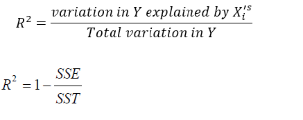
Adjusted R2: To avoid the difficulties of interpreting R2 , the use of adjusted R2 statistics is preferable, defined for a p-term equation as
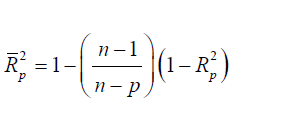
The statistics does not necessarily increase as additional
regressors are introduced into the model, except the partial F- statistic
for testing the significance of the s additional regressors exceeds
one. The criterion for selection of an optimum subset model is to choose the model that has a maximum
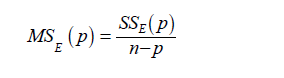
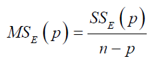
Residual mean square: The residual mean square for a subset residual model may be used as a model evaluation criterion. The MSE(P) experiences an initial decrease, then it stabilizes and eventually may increase as p increases, this is because the sum of square error, SSE(p) always decreases as p increases.
The criterion for selection of an optimum subset model is to choose the model with the following:
a) The minimum
b) The value of p such that is approximately equal to
Note: the subset regression model that minimizes will also maximize
Where
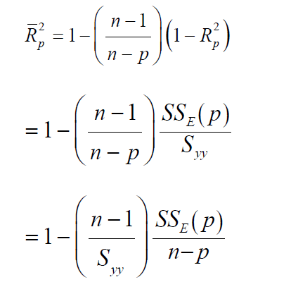
We recall:
Thus, the criteria minimum residual mean square and maximum adjusted coefficient of multiple determinations are equivalent.
Data Analysis and Interpretations
Multiple regression
Regression is a statistical tool for evaluation the relationship between one or more independent variable(s) X1,X2,… X n and a single continuous dependent variable Y. it is most often used when the independent variables are not controllable, that is, when collected in a sample survey or other observational studies. Multiple regression involves more than one independent variables. However, in this work the multiple regression analysis shall consist of seven (7) independent variables, which include; the gross market capitalization, the total new issues, the value of transaction, the market turnover, the total listing of the Nigeria stock market exchange, the All-share index, and the openness of Nigerian Trade Economy. Then the dependent variable is the Gross Domestic Product.
Variable specification
From the data analysis, there are these following variable specifications
Yi=Gross Domestic Product (GDP)
X1=Growth of Market Capitalization
X2=All-share Index
X3=Total Listing on the Nigerian stock exchange
X4=Total New issues
X5=Openness of Nigerian trade Economy
X6=Value of Transaction
X7=Total Market Turnover
Testing for homoscedasticity
Using the scatter plot of the standardized residual against the standardized predictors on all the model obtained by the various variable selection techniques to check for constant variance, we observe that from each chart obtained that only a few points less than four of the residuals vary. This indicates the presence of outliers. But since only few points vary in the entire chart obtained, we can therefore conclude that the residuals have constant variance.
Testing for autocorrelation
Using Durbin Watson d Statistics, we observe that the Durbin Watson d statistic value for the direct search on t, forward selection method, backward elimination method, and the stepwise regression method are 1.049, 0.986, 1.203, and 0.986. since all the values obtained falls within the range 0 and 4, we accept the null hypothesis and conclude that there is no autocorrelation between residuals overtime given by each subset regressor model given by the various techniques.
Obtaining the optimal regression model for the estimation
Here, we have seen independent variables and an optimal regression model is required.

Table 3: Summary of regression coefficients direct search on t.
Using direct search on t: (Table 3) From Table 3, we observe that the regression coefficients of the growth market capitalization, Total listing of the Nigerian stock exchange, Total new issues, value of transaction, and market turnover are 0.001, -42.366, -0.100, 0.003, -53.632 and the probability associated with their t values are all greater than the preselected level of significance 0.05. This indicates that the contribution of the five independent variables to the model is not statistically significant. While the regression coefficient of the All-shares index and the openness of Nigerian trade economy are 9.066 and 11237.220 and the probability associated with their t values are both less than the preselected level of significance 0.05, which shows that the contribution of the All-share index and openness of Nigerian trade economy statistically significant. Therefore, removing the insignificant independent variables, we regressed the gross domestic product on the All-share index and openness of Nigerian trade economy and the model obtained is; GDP=220913.494+4.998ASI+14968.780OTE
Which have a R2 value of 0.958 which shows that 95.8% of the total variation in the real GDP can be explained by the independent variables ASI and OOTE, and an adjusted value of 0.956 and a residual mean square value of 2361918160.279.
Testing for model adequacy:
a) Hypothesis:H0 =The model is not adequate; H1 = The model is adequate. Using a 5% level of significance, (Table 4).

Table 4: Output on test for model adequacy using direct search on t.
b) Interpretation: From the result above with a F-ratio of 333.902 which is significant at 0.000<0.05, we reject the null hypothesis statement that the model is not adequate and conclude that the model is statistically adequate.
Test for parameter significance
a) Hypothesis: 0 H =The parameter is not significant; H1 = The parameter is not significant. Using a 5% level of significance, (Table 5).

Table 5: Summary on the significant regression coefficient using direct search on t.
b) interpretation: From the result, we observed that both independent variables and have unstandardized coefficients of 4.998 and 14968.78 respectively with t-values of 3.513 and 4.770 respectively and are both significant at 0.001<0.05 and 0.000<0.05 respectively. Therefore, we reject the null hypothesis statement that the parameters are not significant and conclude that the parameters are statistically significant.
Using the backward elimination method: Using backward
elimination method, the appropriate model for this analysis, using 
GDP=220550.460+10.593ASI-0.179TNI+10016.59OOTE+0.00 3VALTRANS
R2=0.975 which shows that 97.5% of the total variation in real GDP can be explained by the independent variables ASI, VAL OF TRANS, OOTE, and TNI. With the adjusted R2=0.972 indicating that the fit is good, and residual mean square of 1503272992.23.
Testing for model adequacy
a) Hypothesis: H0 =The model is not adequate; H1 =The model is adequate. Using a 5% level of significance (Table 6)

Table 6: Output on test for model adequacy using backward elimination method.
b) Interpretation: From the result in table 4.5.2.1 above, we observe that with a F-ratio of 266.951 which is significant at 0.000<0.05, we reject the null hypothesis statement that the model is not adequate and conclude that the model is adequate.
Test for parameter significancea) Hypothesis: H0 =The parameter is not significant; H1 = The parameter is significant. Using a 5% level of significance,

Table 7: Summary on the significant regression coefficient using backward elimination method.
b) Interpretation: From the result in the table above, we observed that the independent variablesX2,X4,X5 ,and have coefficients of 10.593, -0.179, 10016.59 and 0.003 respectively with t-values of 5.748, -3.907, 3.601, and 4.024 respectively with p-values all less than 0.05 indicating that the contribution of all the regressors to the model is statistically significant.
Using the Forward Selection Method
Using forward selection method, the appropriate model for this analysis, using a IN F =0.05 is; GDP=223470.496+0.129GMC+0.287ASI+0.622OOTE With a R2=0.968; that is, 96.8% of the total variation in the GDP can be explained by the model.
Testing for model adequacy

Table 8: Output on test for model adequacy using forward selection method.
a) Hypothesis: 0 H =The model is not adequate; H1 = The model is adequate. Using a 5% level of significance (Table 8)
b) Interpretation: From the result in table 4.5.3.1 above, we observe that with a F-ratio of 278.334 which is significant at 0.000<0.05, we reject the null hypothesis statement that the model is not adequate and conclude that the model is adequate.
Test for Parameter Significance
a) Hypothesis:H 0 = The parameter is not significant; H1 = The parameter is significant. Using a 5% level of significance (Table 9)

Table 9: Summary on the significant regression coefficient using forward selection method.
b) Interpretation: From the result in the table above, we observe that ASI, OOTE, and GMC have regression coefficient 3.406, 16315.85, and 0.002 respectively with t values of 2.436, 5.704, 2.814 respectively, with all contributing significantly to the estimates obtained from the model as the estimated values for the dependent variable, since all have p-values less than 0.05, the preselected level of significance.
Using the stepwise regression method: Using stepwise regression method, the appropriate model for this analysis, using FIN=0.05 and FOUT=0.10 is:
GDP=223470.496+0.129GMC+0.287ASI+0.62200TE
With a R2=0.968; that is, 96.8% of the total variation in the GDP can be explained by the model.
Testing for model adequacy
a) Hypothesis: H0 =The model is not adequate; H1 = The model is adequate. Using a 5% level of significance .(Table 10)

Table 10: Output on test for model adequacy using stepwise regression method.
b) Interpretation: From the result in table 4.5.11 above, we observe that the model obtained using the stepwise regression method is also the as that obtained from using the forward selection method, having a F-ratio of 278.334 also which is significant at 0.000<0.05, we reject the null hypothesis statement that the model is not adequate and conclude that the model is adequate.
Test for parameter significance
a) Hypothesis:H0 = The parameter is not significant; H1 = The parameter is significant. Using a 5% level of significance .(Table 11)

Table 11: Summary on the significant regression coefficient using stepwise regression method.
b) Interpretation: From the result in the table above, we observe that ASI, OOTE, and GMC have regression coefficient 3.406, 16315.85, and 0.002 respectively with t values of 2.436, 5.704, 2.814 respectively, with all contributing significantly to the estimates obtained from the model as the estimated values for the dependent variable, since all have p-values less than 0.05, the preselected level of significance
c) Comparing performance of the method (Table12)

Table 12: Ranked Performance of the four variable selection techniques.
selected criteria and obtaining their average rank. We observed that the direct search on t method had an average rank of 3, the forward selection and stepwise regression method both had a tie of 2.5 in their average, and the backward elimination method had an average rank of 1.67.
Using the all possible regression method (Table 13)

Table 13: Ranked Performance of all significant subset models using all possible combination method.
Interpretation: From the result, we observe that according to the Anova tables obtained in the various analyses run on the possible combinations of the seven independent variables, all had P-values for their F-statistics less than the preselected level of significance, thereby indicating that all models are adequate. But using the t-statistic, we observe that some of the models have regression coefficient not significant except the following models with combinations above. In order to obtain the appropriate model for this method, the ranking was used; that is, based on the selected criteria to be used in this analysis. Here judgement is done in this manner; the model with the lowest residual mean square is the best and ranking increases as the residual mean square increases, the one with the lowest VIF is the best and rank increases as VIF increases, while for adjusted R2 the model with the highest adjusted R2is termed best but rank increases with respect to decrease in their respective adjusted R2. And it is summed up as the model combination with the lowest average rank value is termed the best model for estimation. Using this method, the best model using the all possible regression method judging by the average rank is given below as:
GDP=220550.460+10.593ASI-0.179TNI+10016.591OOTE+0.0 03VALTRANS
With a R2 value of 0.975; that is, 97.5% of the total variation in the GDP estimated value can be explained by the model. But taking a good look at the VIF of the model assumed it becomes difficult to make conclusion on this result, it is observed that the VIF is extremely large stating there is a strong presence of multicollinearity, which has a huge effect on precision and confident interval/level.
Conclusion and Recommendation
From the analysis carried out in chapter four on the impact of the Nigerian stock market on her economy development using the various variable selection techniques to obtain models termed best equation based on this technique, the following inferences can be deduced.
Summary
Using direct search on t, ASI and OOTE, that is the All share index (variable 2) and Openness of the Nigerian trade economy (variable 5) respectively, was left in the model as the appropriate subset regressors for the estimation of the Nigerian economy development and growth. The model is found to be adequate using the anova table and it could explain 95.8% of the total variation in the gross domestic of Nigeria. Using the backward elimination method, ASI, OOTE, VALTRANS, and TNI, that is the All-Share index, Openness of the Nigerian trade economy, value of transaction, and total new issues respectively, are left in the model as the appropriate subset regressors for the estimation of the Nigerian economy development and growth. The model is found to be adequate using the anova table and it could explain 97.5% of the total variation in the gross domestic product of Nigerian. Using the Forward selection and stepwise regression method (which is the modified method of the forward selection method). It is observed that both methods gave the same result as the appropriate subset for the estimation; that is, GMC, ASI, and OOTE. The model is found to be adequate using the anova table and it could explain 96.8% of the total variation in the gross domestic product of Nigeria.
Conclusion
From the analysis in chapter four, using the mean rank method to judge for best model, it is observed that backward elimination method gives the best equation for the estimation of the Nigerian gross domestic product with a mean rank of 1.67, wahich is the lowest mean rank. But its variance inflation factor is extremely large indicating strong presence of collinearity amongst some of the independent variables. These could have really affected the signs of the coefficients of the regressors, even if the residual mean square appears to be the lowest compared to other variable selection method. Using the all-possible combination method as a control, as observed in table 4. With a mean rank of 5, the best equation for the estimation is the same as that obtained from the backward selection which contains the; ASI, TNI, VALTRANS, and OOTE as the appropriate subset regressors, using the lowest average rank as the judgement for best model. With a value of 0.975; that is, 97.5% of the total variation in the GDP estimated value can be explained by the model. But taking a good look at the VIF of the model assumed it becomes difficult to make conclusion on this result, it is observed that the VIF is extremely large stating there is a strong presence of multicollinearity, which has a huge effect on precision and confident interval. These contradicts Richard Lockhart’s conclusion that the four variable selection techniques give the same subset model as best.
Recommendation
Although, the variance inflation factor of the regression coefficients was added to the criteria for evaluation of performance, in order to account for the negligence of the effect of multicollinearity before analysis was carried out using the various variable selection techniques. It is advisable for researchers and students, who wants to carry out similar analysis, to ensure that the multicollinearity problem is dealt with in order to satisfy the assumption of no correlation among the independent variables, and researchers can also carry out their finding on other variable selection techniques in regression analysis. A study should also be carried out on the condition in which all four variable selection methods would or would not give the same subset regressor model as best model for estimation.
References
- Montgomery DC, Peck EA (1991) Introduction to linear regression analysis. 2nd Edn pp: 302.
- Efroymson D (1960) Selection of variables in multiple regression part-I. A review and evaluation. Int Statist Rev 46: 1-19.
- Richard Lockhart (2002) Variable selection Method: an introduction. Milano chemometric and QSAR research group, Dept of Environmental sciences, University of Milano, Italy.
- Fan J, R Li (2001) Variable Selection via Nonconcave Penalized Likelihood and its oracle properties. Journal of the America Statistical Association 9(6): 1348-1360.
- Selena NG (2012) Variable Selection in predictive regressions, Department of Economics, Columbia University, New York.
- Wei C (1992) On Predictive Least Squares Principle. Annals of Statistics 20: 1-42.
- Guyon I, A Elisseff (2006) An Introduction to variable and feature selection, Clopinet 955 Creston road, Berkeley, USA.
- Kira K, L Rendell (2006) A practical approach to feature selection. In D Sleeman, P Edwards, editors, international conference on machine learning pp: 368-377.
- Cyprian A Oyeka (2009) An introduction to applied statistical methods, 8th Edn pp: 405.
- Osuji GA, Obubu M, Nwosu CA (2016) Stock Investment Decision in Nigeria; A PC Approach. World Journal of Multidisciplinary and Contemporary Research 2(1): 1-11.
- Osuji GA, Okoro CN, Obubu M, Obiora-Ilouno HO (2016) Effect of Akaike Information Criterion on Model Selection in Analyzing Auto-Crash Variables. International Journal of Sciences 26(1): 98-109.
- Obubu M, Konwe CS, Nwabenu DC, Omokri Peter A, Chijoke M (2016) Evaluation of the Contribution of Nigerian Stock Market on Economic Growth; Regression Approach. European Journal of Statistics and Probability United Kingdom 4(5):11-27.
- Maxwell O, Happiness OI, Alice UC, Chinedu IU (2018) An Empirical Assessment of the impact of Nigerian All Share Index, Market Capitalization and Number of Equities on Gross Domestic Product. Open Journal of Statistics 8(3): 584-602.
- Obubu M, Babalola AM, Ikediuwa CU, Amadi PE (2018) Modeling Count Data; a Generalized Linear Model Framework. American Journal of Mathematics and Statistics 8(6): 179-183.
- Maxwell O, Chukwudike CN, Chinedu OV, Valentine CO, Paul O (2019) Comparison of different Parametric Estimation Techniques in Handing Critical Multicollinearity: Monte Carlo Simulation Study. Asian Journal of Probability and Statistics 3(2): 1-16.
- Maxwell O, Abubarkri OO, Fidelia AI, Joshua IO (2019) Modeling Typhoid Mortality with Box-Jenkins Autoregressive Integrated Moving Average Models. Scholars Journal of Physics, Statistics, Mathematics, p. 6(3): 29-34.


 We use cookies to ensure you get the best experience on our website.